Crossed and Nested hierarchical models with STAN and R

Below I will expand on previous posts on bayesian regression modelling using STAN (see previous instalments here, here, and here). Topic of the day is modelling crossed and nested design in hierarchical models using STAN in R.

Crossed design appear when we have more than one grouping variable and when data are recorded for each combination of the grouping variables. For example say that we measured the growth of a fungi on different Petri dishes and that you took several samples from each dishes. In this example we have two grouping variables: the Petri dish and the sample. Since we have observations for each combination of the two grouping variables we are in a crossed design. We can model this using a hierarchical model with an intercept representing the average growth, a parameter representing the deviation from this average for each Petri dish and an additional parameter representing the deviation from the average for each sample. Below is the corresponding model in STAN code:

/*A simple example of an crossed hierarchical model
*based on the Penicillin data from the lme4 package
*/

data {
  int<lower=0> N;//number of observations
  int<lower=0> n_sample;//number of samples
  int<lower=0> n_plate;//number of plates
  int<lower=1,upper=n_sample> sample_id[N];//vector of sample indeces
  int<lower=1,upper=n_plate> plate_id[N];//vector of plate indeces
  vector[N] y;
}
parameters {
  vector[n_sample] gamma;//vector of sample deviation from the average 
  vector[n_plate] delta;//vector of plate deviation from the average
  real<lower=0> mu;//average diameter value
  real<lower=0> sigma_gamma;//standard deviation of the gamma coeffs
  real<lower=0> sigma_delta;//standard deviation of the delta coeffs
  real<lower=0> sigma_y;//standard deviation of the observations
}
transformed parameters {
  vector[N] y_hat;

  for (i in 1:N)
    y_hat[i] = mu + gamma[sample_id[i]] + delta[plate_id[i]];
}
model {
  //prior on the scale coefficient
//weakly informative priors, see section 6.9 in STAN user guide
  sigma_gamma ~ cauchy(0,2.5);
  sigma_delta ~ cauchy(0,2.5);
  sigma_y ~ gamma(2,0.1);
  //get sample and plate level deviation
  gamma ~ normal(0, sigma_gamma);
  delta ~ normal(0, sigma_delta);
  //likelihood
  y ~ normal(y_hat, sigma_y);
}
generated quantities {
//sample predicted values from the model for posterior predictive checks
  real y_rep[N];
  for(n in 1:N)
    y_rep[n] = normal_rng(y_hat[n],sigma_y);
}

Pasting and saving this code into a .stan file we now turn to R using the Penicillin dataset from the lme4 package as (real-life) example:

library(lme4)
library(rstan)
library(shinystan)#for great model viz
library(ggplot2)#for great viz in general
data(Penicillin)
#look if we have sample for each combination
xtabs(~plate+sample,Penicillin)
#create the plate and sample index
plate_id<-as.numeric(Penicillin$plate)
sample_id<-as.numeric(Penicillin$sample)
#the model matrix (just an intercept in this case)
X<-matrix(rep(1,dim(Penicillin)[1]),ncol=1)

#fit the model
m_peni<-stan(file = "crossed_penicillin.stan",
data=list(N=dim(Penicillin)[1],n_sample=length(unique(sample_id)),
n_plate=length(unique(plate_id)),sample_id=sample_id,
plate_id=plate_id,y=Penicillin$diameter))

#launch_shinystan(m_peni)

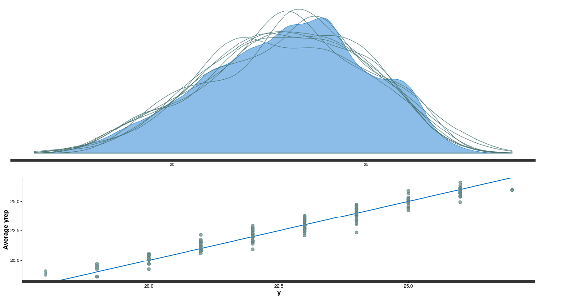
The model seem to fit pretty nicely, all chains converged for all parameters (Rhat around 1), we have decent posterior distribution (top panel in the figure below) and also good correlation between observed and fitted data (bottom panel figure below).

In a next step we can look at the deviation form the average diameter for each sample and each plate (Petri dish):

#make caterpillar plot
mcmc_peni<-extract(m_peni)
sample_eff<-apply(mcmc_peni$gamma,2,quantile,probs=c(0.025,0.5,0.975))
df_sample<-data.frame(ID=unique(Penicillin$sample),Group="Sample",
LI=sample_eff[1,],Median=sample_eff[2,],HI=sample_eff[3,])
plate_eff<-apply(mcmc_peni$delta,2,quantile,probs=c(0.025,0.5,0.975))
df_plate<-data.frame(ID=unique(Penicillin$plate),Group="Plate",
LI=plate_eff[1,],Median=plate_eff[2,],HI=plate_eff[3,])
df_all<-rbind(df_sample,df_plate)
ggplot(df_all,aes(x=ID,y=Median))+geom_point()+
 geom_linerange(aes(ymin=LI,ymax=HI))+facet_wrap(~Group,scales="free")+
 geom_hline(aes(yintercept=0),color="blue",linetype="dashed")+
 labs(y="Regression parameters")

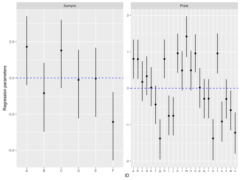
We can compare this figure to Figure 2.2 in here where the same model was fitted to the data using lmer.

I now turn to nested design. Nested design occur when there is more than one grouping variable and when there is a hierarchy in these variables with categories from lower variables only being present at one level from higher variables. For examples if we measured student scores within classes within schools we would have a nested hierarchical design. In the following I will use the Arabidopsis dataset from the lme4 package. Arabidopsis plants from different regions (Netherlands, Spain and Sweden) and from different populations within these regions (nested design) were collected and the researchers looked at the effect of herbivory and nutrient addition on the number of fruits produced per plants. Below is the corresponding STAN code:

/*Nested regression example
*Three-levels with varying-intercept
*based on: https://rpubs.com/kaz_yos/stan-multi-2
*and applied to the Arabidopsis data from lme4
*/

data {
  int<lower=1> N; //number of observations
  int<lower=1> P; //number of populations
  int<lower=1> R; //number of regions
//population ID
  int<lower=1,upper=P> PopID[N]; 
 //index of population appertenance to a specific region
  int<lower=1,upper=R> PopWithinReg[P]; 

  int<lower=0> Fruit[N]; //the response variable
  real AMD[N]; //predictor variable, whether the apical meristem was unclipped (0) or clipped (1)
  real nutrient[N]; //predictor variable, whether nutrient level were control (0) or higher (1)
}

parameters {
  //regression slopes
  real beta_0; //intercept
  real beta_1; //effect of clipping apical meristem on number of fruits
  real beta_2; //effect of increaing nutrient level on number of fruits

  //the deviation from the intercept at the different levels
  real dev_pop[P]; //deviation between the populations within a region
  real dev_reg[R]; //deviation between the regions

  //the standard deviation for the deviations
  real<lower=0> sigma_pop;
  real<lower=0> sigma_reg;
}

transformed parameters {
  //varying intercepts
  real beta_0pop[P];
  real beta_0reg[R];

  //the linear predictor for the observations
  real<lower=0> lambda[N];

  //compute the varying intercept at the region level
  for(r in 1:R){
    beta_0reg[r] = beta_0 + dev_reg[r];}

  //compute varying intercept at the population within region level
  for(p in 1:P){
     beta_0pop[p] = beta_0reg[PopWithinReg[p]] + dev_pop[p];}

  //the linear predictor
  for(n in 1:N){
     lambda[n] = beta_0pop[PopID[n]] + beta_1 * AMD[n] + beta_2 * nutrient[n];}
}

model {
  //weakly informative priors on the slopes
  beta_0 ~ cauchy(0,5);
  beta_1 ~ cauchy(0,5);
  beta_2 ~ cauchy(0,5);

  //weakly informative prior on the standard deviation
  sigma_pop ~ cauchy(0,2.5);
  sigma_reg ~ cauchy(0,2.5);

  //distribution of the varying intercept
  dev_pop ~ normal(0,sigma_pop);
  dev_reg ~ normal(0,sigma_reg);

  //likelihood
  Fruit ~ poisson_log(lambda);
}

generated quantities {
//sample predicted values from the model for posterior predictive checks
 int<lower=0> fruit_rep[N];
 for(n in 1:N)
   fruit_rep[n] = poisson_log_rng(lambda[n]);
}

I decided to use a Poisson distribution as the response is a count variable. The only “tricky” part is the index linking a particular population to its specific region (PopWithinReg). In this model we assume that variations between populations within regions is only affecting the average number of fruits but is not affecting the plant responses to the simulated herbivory (AMD) and to increased in nutrient levels. In other words populations within region is an intercept-only “random effect”. We turn back to R:

 data("Arabidopsis")
#generate the IDs
pop.id <- as.numeric(Arabidopsis$popu)
pop_to_reg <- as.numeric(factor(substr(levels(Arabidopsis$popu),3,4)))
#create the predictor variables
amd <- ifelse(Arabidopsis$amd=="unclipped",0,1)
nutrient <- ifelse(Arabidopsis$nutrient==1,0,1)

m_arab <- stan("nested_3lvl.stan",data=list(N=625,P=9,R=3,PopID=pop.id,
PopWithinReg=pop_to_reg,Fruit=Arabidopsis$total.fruits,
AMD=amd,nutrient=nutrient))
#check model
#launch_shinystan(m_arab)

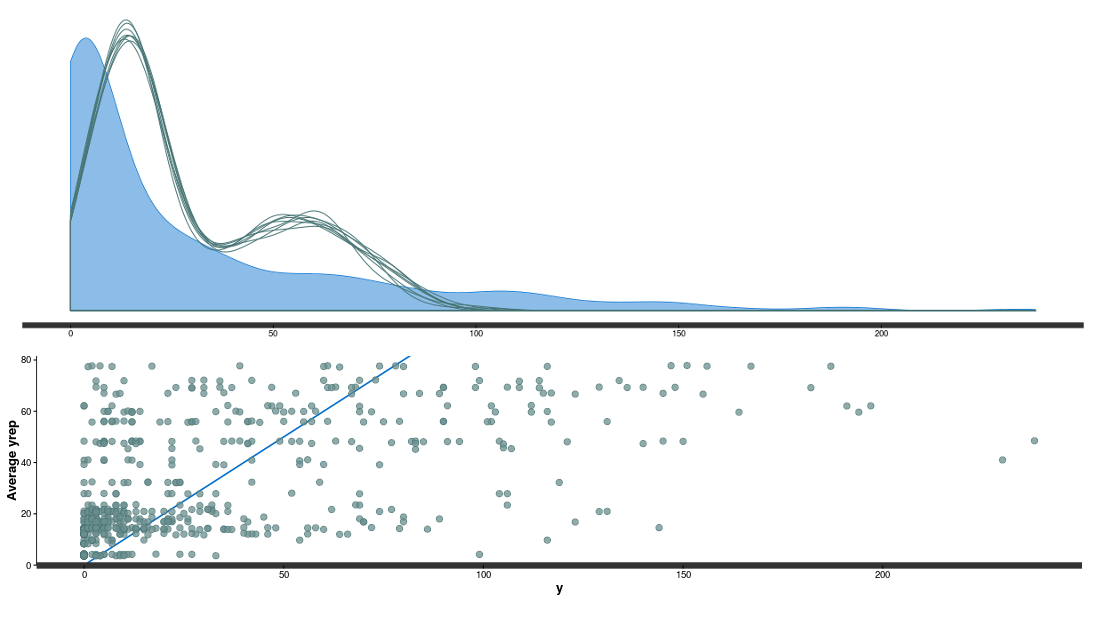
Rstan is warning us that we had some divergent iterations, we could correct this using non-centered re-parametrization (See this post and the STAN user guide). More worrisome is the discrepancy between the posterior predictive data and the observed ones:

We can explore these errors for each populations within regions:

mcmc_arab <- extract(m_arab)
#plot obs vs fitted data across groups
fit_arab <- mcmc_arab$fruit_rep
#average across MCMC samples
Arabidopsis$Fit <- apply(fit_arab,2,mean)
#plot obs vs fit
ggplot(Arabidopsis,aes(x=total.fruits,y=Fit,color=amd,shape=factor(nutrient)+
geom_point()+facet_wrap(~popu,scales="free")+
geom_abline(aes(intercept=0,slope=1))

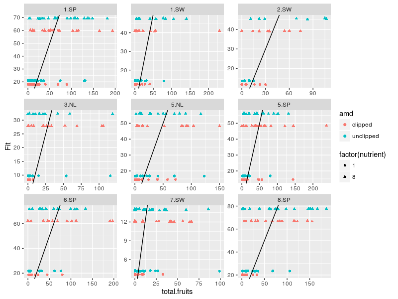
The model predict basically four values, one for each combination of the two treatment variables. The original data are way more dispersed than the fitted ones, one could try to use negative binomial distribution while making the treatment effect also vary between the populations between the regions …

That’s it for this post, a great source of regression models for further examples in the STAN-wiki.