Spatial Dynamic in a Host-Parasitoid system

In this post I will explore the spatial dynamic that arise from a simple deterministic host-parasitoid model with migration in a homogeneous environment. If the previous sentence did not drive you away, congrats (!) you are most certainly in a terminal state towards biological nerditude.

The idea of this post emerged while reading Chp. 6 in Hanski and Gilkin Metapopulation book. In this Chapter Nay and colleagues expand the classical one-species metapopulation models to models with interacting species. In one example they talk about their 1992 paper where they took a simple Host-Parasitoid system and applied this in a metapopulation context where local populations (a patch) are linked by migrations between adjacent patches. Their main results is that a system that is unstable in a single local population become stable at the metapopulation level (does this sounds familiar?). In other words, local host-parasitoid system that alone show extinction, present persistence of both species when local populations exchange migrants. Pretty cool stuff, of course along the way they also show some beautiful spatial patterns, but that is secondary (isn’t it?).

Here is the model:

$latex N_{i,t} = J_{i,t-1}    e^{-aP_{i,t-1}}$

$latex Q_{i,t} = c * (J_{i,t-1} - N_{i,t})$

$latex J_{i,t} = \lambda * (N_{i,t} * (1 - \mu_{n}) + \mu_{n}  * \sum_{j=1}^{8} \frac{N_{j,t}}{8})$

$latex P_{i,t} = Q_{i,t} * (1 - \mu_{q}) + \mu_{q}  * \sum_{j=1}^{8} \frac{Q_{j,t}}{8}$

Where N is the abundance of the pre-dispersal hosts, Q is the abundance of pre-dispersal parasitoid , J is the abundance of post-dispersal hosts, P is the abundance of post-dispersal parasitoid. i is an index for the patches, t is the time, j is an index for the patches that are neighbouring patch i (we consider here only the direct neighbour). a is the searching efficiency of the parasitoid, c is the number of parasitoid per hosts, $latex \lambda$ is the host growth rate, and the $latex \mu$ are the migration rate for the host (n) and for the parasitoid (q).

Got it? Now let’s code this into R:

#Local dynamics following Nicholson-Bailey 
#host-parasitoid function with one parameter: a
#@J: matrix of juvenil abundance in the previous time step
#@P: number of adult parasitoid in the previous time step
#@a: the searching efficiency of the parasitoid
#@c: the number of parasitoid per hosts
local_dyn<-function(J,P,a=0.1,c=1){
  N <- J*exp(-a*P)
  Q <- c*(J - N)
  return(list(N=N,Q=Q))
}




#an helper function returning line numbers of all neighbouring cells
find_neighbour<-function(vec,dat=dat){
  lnb<-which(dat[,"x"]%in%(vec["x"]+
c(-1,-1,-1,0,1,1,1,0)) & dat[,"y"]%in%(vec["y"]+c(-1,0,1,1,1,0,-1,-1)))
  #remove own line
  lnb<-lnb[which(lnb!=vec["lnb"])]
  return(lnb)
}




#compute the next-generation parasitoid and hosts
#with immigration and absorbing boundaries
#@N: matrix of adult host in the current generation
#@Q: matrix of emerging parasitoid in the current generation
#@neigh: a list with the cell ID of neighbouring cells
#@mu: immigration rates
#@lbd: rate of increase of host population
#@bound: type of boundaries, either absorbing where individuals
#are lost from the systemat the boundaries or reflective where
#individuals are not able to leave the system
imm_dyn <- function(N,Q,neigh,mu_n=0.5,mu_q=0.5,lbd=2,bound="absorbing"){
  if(bound=="absorbing"){
    J <- lbd*(N*(1-mu_n) + mu_n*laply(neigh,function(x) sum(N[x]/8)))
    P <- Q*(1-mu_q) + mu_q*laply(neigh,function(x) sum(Q[x]/8))
  }
  else if(bound=="reflective"){
    J <- lbd*(N*(1-mu_n) + 
mu_n*laply(neigh,function(x) sum(N[x]/dat$Nb[dat$lnb%in%x])))
    P <- Q*(1-mu_q) + 
mu_q*laply(neigh,function(x) sum(Q[x]/dat$Nb[dat$lnb%in%x]))
  }
  else{
    print("Boundary type provided is not implemented yet")
    break
  }
  return(list(J=J,P=P))
}

Here are three functions, the first one implement the local host-parasitoid dynamic, the second one is just an helper function to get the cell ID of neighbouring cells and the third one implement the migration between neighbouring cells. A critical point in spatially-explicit models is boundary behaviour. A boundary can either be absorbing: modelled entities are able to leave the simulated system, and when they do they are lost; circular: modelled entities are able to leave the system and when they do they re-enter the system at the opposite end (ie the system is a sphere); reflective: modelled entities cannot leave the system. Here I implement absorbing (hosts or parasitoids are leaving the metapopulation) and reflective (hosts are parasitoids are “afraid” to leave the metapopulation) boundaries.

Simulation time:

#load the libraries
library(plyr) #for data wraggling
library(reshape2) #for melting
library(ggplot2) #for nice graphs
library(viridis) #for nice colors
#set up seed
set.seed(20161211)
#set up number of generations and grid size
generation<-1:100
n_x <- n_y <- 30
#representation of the grid
dat<-expand.grid(x=1:n_x,y=1:n_y)
dat$lnb<-1:(n_x*n_y)
#create a list where each element contain the cell ID 
#of the neighbour of the focal cell
neigh<-apply(dat,1,function(x) find_neighbour(x,dat))
#compute the number of neighbours for each cells to use 
#in reflective boundaries
dat$Nb<-laply(neigh,length)




#set the object keeping the dynamic and the initial condition
Js <- array(0,dim=c(30,30,101))
Ps <- array(0,dim = c(30,30,101))
#host and parasitoid start at one cell
Js[15,15,1] <- rpois(n=1,lambda=5)
Ps[15,15,1] <- rpois(n=1,lambda = 2)




#simulation
for(i in generation){  
  tmp <- local_dyn(J = Js[,,i],P = Ps[,,i],a=1)
  tmp2 <- imm_dyn(N = tmp[["N"]],Q = tmp[["Q"]],
    neigh = neigh,lbd=2,bound="absorbing")
  Js[,,(i+1)] <- tmp2[["J"]]
  Ps[,,(i+1)] <- tmp2[["P"]]
  print(i)
}




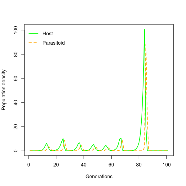
#plot temporal dynamic for one patch
plot(1:101,Js[20,15,],type="l",lwd=2,col="green",
  xlab="Generations",ylab="Population density")
lines(1:101,Ps[20,15,],lty=2,lwd=2,col="orange")
legend("topleft",c("Host","Parasitoid"),lwd=2,
  lty=c(1,2),col=c("green","orange"),bty="n")

#temporal dynamic accros one transect from the center outwards
tra<-Js[15:30,15,]
tram<-melt(tra,value.name = "Pop")
names(tram)[1:2]<-c("Cell","Gen")
ggplot(tram,aes(x=Gen,y=Pop,color=factor(Cell),group=Cell))+geom_line()+
  labs(x="Generation",y="Population density")

This is actually pretty interesting, we see the wave of colonisation from the original cell (N° 1) up to the edge of the simulated system (cell N° 16), the first wave is pretty well ordered from 1-16 but then at generation 25, cells in the middle peak a bit earlier as the one in the center, and this is then amplified for the next peaks at generation 40 and 50.

#Phase space plot for average densities
ph<-data.frame(Gen=1:101,Host=log(apply(Js,3,mean)),
  Parasitoid=log(apply(Ps,3,mean)))
ggplot(ph,aes(x=Host,y=Parasitoid))+geom_path()+
  geom_label(aes(label=Gen))

This graphs show the dynamics of  host-parasitoid average densities, it reveals among other things that we have cycles of varying amplitude.

#look at spatial dynamic for host and parasitoid
#between generations 50 and 53
exmpl<-data.frame(Gen=rep(50:53,each=900),x=rep(rep(1:30,times=30),4),
 y=rep(rep(1:30,each=30),4),Host=as.numeric(Js[,,50:53]),
 Parasitoid=as.numeric(Ps[,,50:53]))
exmplm<-melt(exmpl,id.vars=c("x","y","Gen"),variable.name="Species",
  value.name="Pop")
ggplot(exmplm,aes(x,y,fill=Pop))+geom_raster(interpolate=TRUE)+
  scale_fill_viridis(option="plasma",direction=-1)+
  facet_grid(Gen~Species)+labs(x="",y="")+
  theme(axis.text=element_text(size=0),axis.ticks.length=unit(0,"cm"))

Pretty nice! Now let’s do the same simulations but this time with reflective boundaries, ie host and parasitoid cannot leave the system:

#make the boundary reflective
Js2 <- array(0,dim=c(30,30,101))
Ps2 <- array(0,dim = c(30,30,101))
#host and parasitoid start at one cell
Js2[15,15,1] <- rpois(n=1,lambda=5)
Ps2[15,15,1] <- rpois(n=1,lambda = 2)

for(i in generation){  
  tmp <- local_dyn(J = Js2[,,i],P = Ps2[,,i],a=1)
  tmp2 <- imm_dyn(N = tmp[["N"]],Q = tmp[["Q"]],neigh = neigh,lbd=2,
    mu_n=0.5,mu_q=0.5,bound="reflective")
  Js2[,,(i+1)] <- tmp2[["J"]]
  Ps2[,,(i+1)] <- tmp2[["P"]]
  print(i)
}

#Phase space plot for average densities
ph<-data.frame(Gen=1:101,Host=log(apply(Js2,3,mean)),
  Parasitoid=log(apply(Ps2,3,mean)))
ggplot(ph,aes(x=Host,y=Parasitoid))+geom_path()+
  geom_label(aes(label=Gen))

Again cycling of host-parasitoid densities with changing amplitude.

#spatial patterns
exmpl<-data.frame(Gen=rep(75:78,each=900),x=rep(rep(1:30,times=30),4),
  y=rep(rep(1:30,each=30),4),Host=as.numeric(Js2[,,75:78]),
  Parasitoid=as.numeric(Ps2[,,75:78]))
exmplm<-melt(exmpl,id.vars=c("x","y","Gen"),
  variable.name="Species",value.name="Pop")
ggplot(exmplm,aes(x,y,fill=Pop))+geom_raster(interpolate=TRUE)+
  scale_fill_viridis(option="magma",direction=-1)+
  facet_grid(Gen~Species)+labs(x="",y="")+
  theme(axis.text=element_text(size=0),axis.ticks.length=unit(0,"cm"))

Using ImageMagick and its function convert one can easily turn this into an animated GIFs to observe the whole dynamic.

Why bothering about all this? Developing such models reveal that depending on the size of the system (the number of patch), the metapopulation of hosts and parasitoid may persist or not. In other words if we reduce the size of natural habitat a host-parasitoid system that was persisting through time despite large variations might suddenly be driven to extinction.