Fitting scale-dependent landscape effect with greta

A large number of ecological processes depend not only on the local conditions but also on the surrounding landscape. Think of birds being measured at a number of focal sites, the number of birds observed at these sites will depend on the land-use in the surrounding landscape. To link these site-based measures with the landscape, a common approach is to draw a serie of concentric rings around the site, to measure a variable of interest (like percent of grassland cover) and to fit separate models for each ring selecting the one providing the best fit (see top panel of figure below).

This approach assume consistent landscape effect up to a certain threshold and no landscape effect beyond this threshold. Another, conceptually more satisfaying approach, is to assume a distance-decay of a given form of the landscape effect (see bottom panel of figure). With this approach the different rings are weighted based on their radius, smaller rings having more weight than bigger rings, with the model estimating how fast the landscape effect decay with ring size.

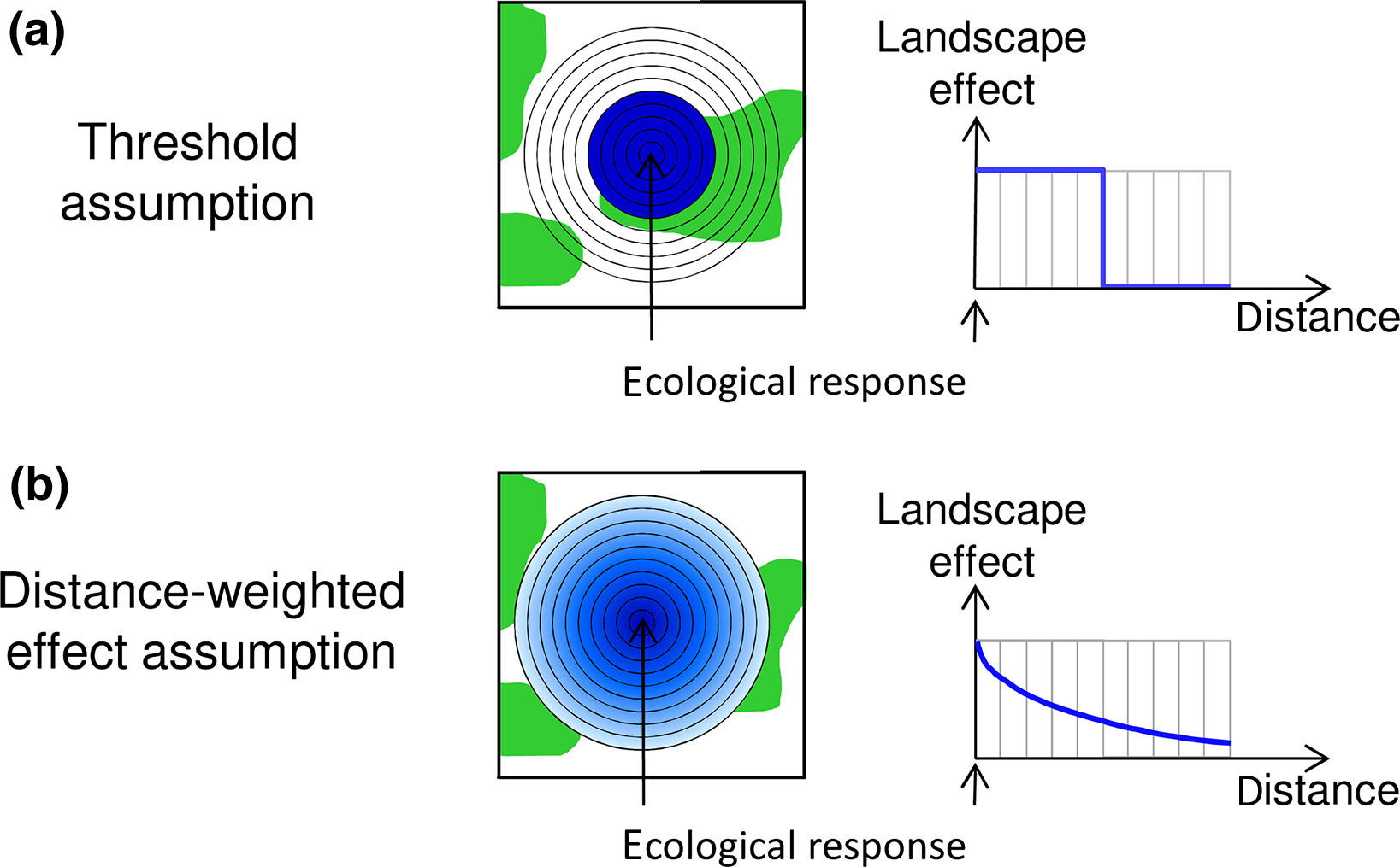
Figure from Miguet et al 2017: https://doi.org/10.1111/2041-210X.12830

With the distance-decay approach one need to define a decay or weight function, for this post we will use the following half-normal kernel:

\[w_i = e^{- \frac{r_i ^ 2}{2 * \delta ^ 2}}\]

where w is the weight attributed to a ring i, r is the radius of the ring and \(\delta\) is the decay parameter to be estimated by the model.

The next step is to turn the weight function into a distance function:

\[d_i = \frac{w_i * a_i}{\sum_i w_i * a_i}\]

where a is the area of the ring (note that this can be extended to cases where the area of the ring differ between the observation). The division is to ensure that the distance weight sum to one.

Then we can derive the covariate as follow:

\[x_j = \sum_i d_i * X_{ij}\]

where X is a matrix with i columns (one for each ring) and j rows (one for each observations).

The weighed covariate can then be plugged into a classical regression framework such as:

\[y \sim \mathcal{N}(\beta_0 + \beta_1 * x, \sigma)\]

So we have the theory in place, let’s see how to fit such a model in greta (check this website for infos on the package), we will use for this a simulated dataset the you can generate following the code at the end of the post.

# load libraries
library(greta)
library(ggplot2)

# look at the data
str(dat)

Classes ‘tbl_df’, ‘tbl’ and 'data.frame':	100 obs. of  23 variables:
 $ ID      : int  1 2 3 4 5 6 7 8 9 10 ...
 $ X_1     : num [1:100, 1] 0.0112 0.0902 0.0419 0.6409 0.6409 ...
 $ X_12    : num [1:100, 1] 0.0277 0.2012 0.4672 0.6696 0.6409 ...
 $ X_23    : num [1:100, 1] 0.197 0.282 0.556 0.722 0.525 ...
 $ X_34    : num [1:100, 1] 0.285 0.374 0.593 0.574 0.451 ...
 $ X_45    : num [1:100, 1] 0.347 0.418 0.643 0.49 0.408 ...
 $ X_56    : num [1:100, 1] 0.407 0.452 0.634 0.46 0.439 ...
 $ X_67    : num [1:100, 1] 0.445 0.46 0.561 0.444 0.426 ...
 $ X_78    : num [1:100, 1] 0.447 0.459 0.507 0.421 0.428 ...
 $ X_89    : num [1:100, 1] 0.457 0.459 0.464 0.437 0.44 ...
 $ X_100   : num [1:100, 1] 0.459 0.459 0.452 0.454 0.448 ...
 $ area_1  : num  3.14 3.14 3.14 3.14 3.14 ...
 $ area_12 : num  452 452 452 452 452 ...
 $ area_23 : num  1661 1661 1661 1661 1661 ...
 $ area_34 : num  3630 3630 3630 3630 3630 ...
 $ area_45 : num  6359 6359 6359 6359 6359 ...
 $ area_56 : num  9848 9848 9848 9848 9848 ...
 $ area_67 : num  14096 14096 14096 14096 14096 ...
 $ area_78 : num  19105 19105 19105 19105 19105 ...
 $ area_89 : num  24873 24873 24873 24873 24873 ...
 $ area_100: num  31402 31402 31402 31402 31402 ...
 $ pred    : num  0.0926 0.2328 0.4974 0.6836 0.5959 ...
 $ resp    : num  2.64 2.29 6.65 7.6 7.82 ...

The dataset contain 10 columns with the covariate values in rings of increasing size from 1 to 100, the 10 next columns are the areas of these rings, the column “resp” contain the response values.

We can now develop the model via the following steps: (i) define prior distributions for all model parameters, (ii) define the weight and the distance function, (iii) compute the covariate, (iv) define the linear predictor and the likelihood.

# modelling part
## first generate the priors
# priors on parameters
beta_0 <- student(3, 0, 10) # intercet
beta_1 <- normal(0, 1) # slope
sdd <- gamma(0.01, 0.01) # residual deviation
rate_e <- exp(student(3, 0, 10)) # decay of effect

# build the weights
w_f <- exp(- (rad ** 2) / (2 * rate_e ** 2))
# build the distance function
# by multiplying with the ring area
d_f <- sweep(t(dat[,12:21]), 1, w_f, FUN = "*")  
# scale the distance function so that the rows sum to one
d_fscale <- sweep(t(d_f), 1, greta::colSums(d_f), FUN = "/")
# build the predictor
X <- greta::rowSums(as.matrix(dat[,2:11]) * d_fscale)
# the linear predictor
mu <- beta_0 + beta_1 * X

# the likelihood
y <- as_data(dat$resp)
distribution(y) <- normal(mu, sdd)

# the model
m <- model(beta_0, beta_1, sdd, rate_e)
# sample the posterior
dd <- mcmc(m, hmc(Lmin = 30, Lmax = 35), one_by_one = TRUE)

Once the model was fitted we do some standard model checks:

# Rhat
coda::gelman.diag(dd)

Potential scale reduction factors:

       Point est. Upper C.I.
beta_0          1       1.00
beta_1          1       1.01
sdd             1       1.01
rate_e          1       1.00

Multivariate psrf

1

# posterior predictive distribution
greta.checks::pp_check(dd, y, nsim = 50)

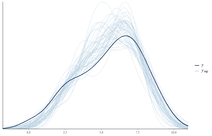
For more about post-fitting checks for greta, you can check this post.

From the fitted model we can derive a couple of interesting plots such as the estimated distance function:

# new radius and weights that are more precise
rad_n <- seq(min(rad), max(rad), 1)
surf_n <- pi * rad_n ** 2
w_fn <- exp(- (rad_n ** 2) / (2 * rate_e ** 2))
# get the distance weight function assuming perfect circles
dw_n <- (w_fn * surf_n) / sum(w_fn * surf_n)
# get posterior draw from this
dw_post <- as.matrix(calculate(dw_n, values = dd))
# plot some of these distance function
plot(rad_n, dw_post[1,], col = "lightblue", lty = 2, type = "l",
     ylim = c(0, 0.15), xlab = "Radius", ylab = "Weight")

# plot a couple of posterior draws
rnd <- sample(2:4000, 25, replace = FALSE)
for(i in rnd){
  lines(rad_n, dw_post[i,], col = "lightblue", lty = 2)
}

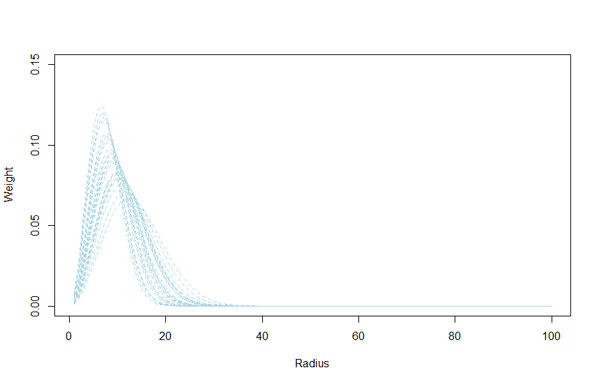
From this graph we can see that landscape conditions beyond 40 have little effect on the response.

We can derive two interesting parameters: (i) the radius with the largest effect, or in other word which circle has the most influence on the response and (ii) the radius at which 90% of the effect is reached, or in other word the distance at which 90% of the landscape effect happens.

# find the distance with max value
scale_max <- rad_n[apply(dw_post, 1, which.max)]
# find the distance with 90% of the effect
# an helper function to do that
find_90 <- function(x){
  cc <- cumsum(x)
  which.min(abs(cc - 0.9))
}

scale_90 <- rad_n[apply(dw_post, 1, find_90)]

# plot the 95% CrI of these two parameters
pars <- data.frame(var = c("scale_max", "scale_90"),
                   med = c(median(scale_max), median(scale_90)),
                   lci = c(quantile(scale_max, probs = 0.1),
                           quantile(scale_90, probs = 0.1)),
                   uci = c(quantile(scale_max, probs = 0.9),
                           quantile(scale_90, probs = 0.9)))
ggplot(pars, aes(x=var, y=med, ymin=lci, ymax=uci)) +
  geom_linerange() +
  geom_point() +
  coord_flip() +
  labs(x = "Parameter",
       y = "Radius")

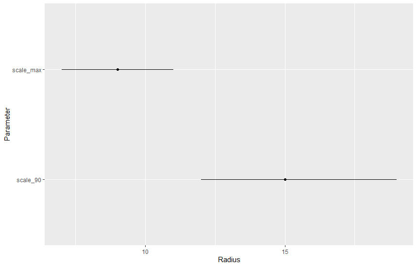
The largest landscape effects are around 8, while 90% of the landscape effect was reached at 15.

To plot the effect of the landscape covariates one can either create spatially explicit scenarios of changes and re-compute all the buffers, or one can just plot the predicted regression line along the gradient of observed covariate values, we will see the second option:

# create a new covariate
x_new <- seq(min(dat[,2:11]), max(dat[,2:11]), length.out = 10)
# the linear predictor
mu_new <- beta_0 + beta_1 * x_new
# compute posterior draws
pred <- as.matrix(calculate(mu_new, values = dd))
# put together for plotting
pred_df <- data.frame(x = x_new,
                      med = apply(pred, 2, median),
                      lci = apply(pred, 2, quantile, probs = 0.1),
                      uci = apply(pred, 2, quantile, probs = 0.9))


ggplot(pred_df, aes(x=x, y=med, ymin=lci, ymax=uci)) +
  geom_ribbon(alpha = 0.2) +
  geom_line() +
  labs(x = "Landscape covariate",
       y = "Predicted response")

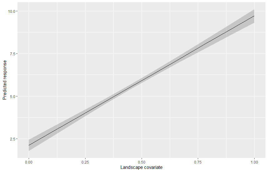
In this post we saw how to estimate landscape-scale effect on variables measured at various sites by explicitely taking into account the fact that conditions close to the site have more importance than conditions far away. The distance decay estimated with this model can have practical implication for instance in revealing how landscapes should be managed in order to optimize the response.

Here we only had a simple model with one covariate, this can of course be extended by adding more covariates with or without distance decay effect.

Some handy references:

• Miguet et al 2017
• Moll et al 2020

Below is the code to simulate the dataset:

# data simulation part
library(NLMR)
library(raster)
library(sf)
library(dplyr)
library(tidyr)
# an agri landscape
agri <- nlm_randomrectangularcluster(100, 100, minl = 10, maxl = 50)
# now the points of obs
dat <- data.frame(x = runif(100, 0, 100),
                  y = runif(100, 0, 100))
dat_sf <- st_as_sf(dat, coords = c("x", "y"))
# augment
dat_sfb <- dat_sf[rep(1:100, each = 10),]
dat_sfb$radius <- rep(seq(1, 100, length.out = 10), 100)
# compute the buffer
buffer <- st_buffer(dat_sfb, dat_sfb$radius)
# compute the mean value within the buffer
buffer$X <- raster::extract(agri, buffer, fun = mean)
# get the area
buffer$area <- st_area(buffer)
names(buffer)[2] <- "radius"
# widen up
buffer %>%
  as_tibble() %>%
  dplyr::select(radius, X, area) %>%
  mutate(ID = rep(1:100, each = 10)) %>%
  pivot_wider(names_from = radius, values_from = c(X, area), id_cols = ID) -> dat

# get the weight
rad <- seq(1, 100, length.out = 10)
w <- exp(- (rad ** 2) /(2 * 10 ** 2))
# the distance function
dw <- sweep(dat[, 12:21], 2, w, FUN = "*")
# scale per row
dw_scale <- dw / base::rowSums(dw)

# generate the predictor
dat$pred <- base::rowSums(dat[,2:11] * dw_scale)
# simulate some response
dat$resp <- rnorm(100, 1 + 10 * dat$pred, 1)