Recurrent themes in my work: covariance

Some themes keeps popping up in different projects or aspects of my work and I would like to reflect a bit on them in a series of posts.

In this first post on recurrent themes I will explore covariance matrices, what they are, when they appear and how to use them. This last part will include some R code so that you can try things out.

What is a covariance matrix?

A covariance matrix is an ordered collection of covariance between a group of variables. Covariance is always defined between two variables, it measures how much the two variables are moving together. Positive covariance means that when values of one variables get high, the values of the other variables also get high. Negative covariance means that when one variable is increasing the other is decreasing. This sounds pretty much like correlation. This is because correlation is the scaled covariance, in other words covariance can go from -Inf up to +Inf, correlation is constrained between -1 and 1. In more mathematical terms we have:

\[Cov(X, Y) = \frac{\sum_{i=1}^{N} (X_i - \bar{X}) * (Y_i - \bar{Y})}{N - 1}\]

for the covariance, with the \(\bar{X}\) representing the mean X value and

\[Cor(X, Y) = \frac{Cov(X, Y)}{\sigma_X * \sigma_Y}\]

for the correlation where the \(\sigma\) are the standard deviation of the variables.

So covariance is unit-dependent, if you measure the covariance between a variable in meter and a variable in gramm you will get a covariance value in metergramm, turning these variables into km and kg will get you different covariance. On the other hand correlations are unitless, so you can apply any linear transformation to your data and the correlation will remain constant. In other words covariance might be trickier to interpret than correlation.

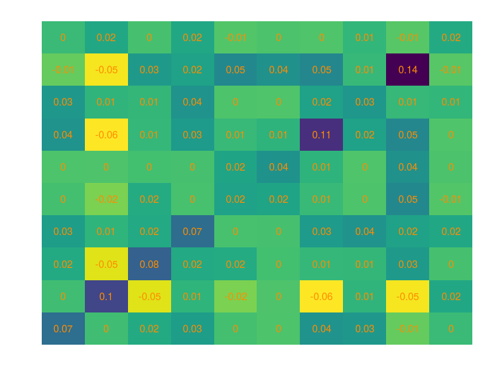
Below is how a covariance matrix could look like:

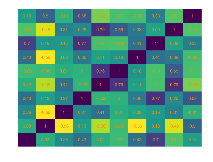
And the corresponding correlation matrix

When can you expect covariance matrices to creep in?

Covariance matrices come along the way in every instance where you model relationships between variables or data points. For instance in GLMMs the random effects on the same grouping variables are expected to be correlated and the model is internally using covariance matrices to estimate these correlations. Here is a short R example

library(nlme)
library(lme4)
data("Orthodont")
lmer(distance ~ age + Sex + (age | Subject), Orthodont)

Linear mixed model fit by REML ['lmerMod']
Formula: distance ~ age + Sex + (age | Subject)
   Data: Orthodont
REML criterion at convergence: 435.2339
Random effects:
 Groups   Name        Std.Dev. Corr 
 Subject  (Intercept) 2.7970        
          age         0.2264   -0.77
 Residual             1.3100        
Number of obs: 108, groups:  Subject, 27
Fixed Effects:
(Intercept)          age    SexFemale  
    17.6352       0.6602      -2.1455  

The important part there is the Corr information, the model tell us that there is a negative covariance between the varying intercept and the varying slope, in more biological terms subjects with higher distance will tend to have lower age slopes.

Another modelling approach that intensively use covariance matrix is structural equation modelling. In structural equation models relationships between variables are estimated from patterns in the covariance. Basically the covariance between a pair of variables is expressed in terms of their hypothetical relations. Some algorithm is then running trying to best accommodate hypothetical relations and observed covariance matrices and if the two are pretty close then the model does a good job of extracting the relation between the variables.

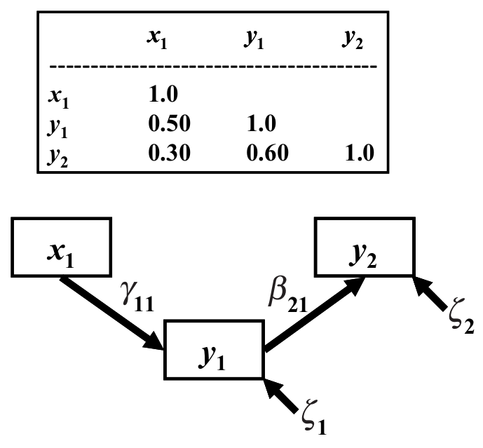
From James Grace: Structural Equation Modeling and Natural Systems, Cambridge University Press

A final place where covariance matrices pop in is when independence of the residuals is violated by some kind of temporal or spatial relations (whether this is always a bad thing is discussed here). One way to take these components into account is by allowing errors to covary following some kind of functions. For spatial or photogenically-correlated errors the idea is then to make the covariance between two data points depend on the spatial or phylogenetic distance between the two points. In R such models can be ran via MCMCglmm, INLA, gstat or other packages.

Some properties of covariance matrices

Covariance matrices have a few distinctive features that I will outline below:

• square: covariance matrices have as many rows as columns, remember each entry in the covariance matrix is the covariance between two variables

• diagonal: the diagonal elements in the covariance matrix are the variances of the variables, go back to the formula at the beginning and replace X1 and X2 by X and you will see the variance formula in front of your eyes

• symmetric: covariance matrix are symmetric based on the diagonal, the covariance between A et B is the same as the covariance between B and A, again looking at the formula this makes sense. For large datasets and complex models this usually means that we do not need to carry the full covariance matrix around, the lower or upper triangle is enough

• positive definitiveness: covariance matrix MUST be positive definitive, this means that multiplying a matrix that is positive-definite by any non-zero vector will always return a positive number. This is a bit of a pain when you want to simulate stuff and you have to generate covariance matrices, you cannot just simulate any numbers, some kind of structure as to be present (but see this entry which show some code to randomly generate covariance matrices).

• cholesky decomposition: this is a cool trick to pass around the positive definitiveness issue, a positive definite matrix can be cholesky decompose into a lower-triangle matrix that when multiplied with its transpose returns the covariance matrix. This is a neat trick to optimize typical Monte Carlo sampling but also least squares problems.