Hierarchical models with RStan (Part 1)

Real-world data sometime show complex structure that call for the use of special models. When data are organized in more than one level, hierarchical models are the most relevant tool for data analysis. One classic example is when you record student performance from different schools, you might decide to record student-level variables (age, ethnicity, social background) as well as school-level variable (number of student, budget). In this post I will show how to fit such models using RStan. As there is much to say and try on such models I restrict myself in this post to a rather simple example, I will extend this to more complex situations in latter posts.

A few words about RStan:

If you don’t know anything about STAN and RStan make sure to check out this webpage. In a few words RStan is an R interface to the STAN programming language that let’s you fit Bayesian models. A classical workflow looks like this:

1. Write a STAN model file ending with a .stan

2. In R fit the model using the RStan package passing the model file and the data to the stan function

3. Check model fit, a great way to do it is to use the shinystan package

First example with simulated data:

Say that we recorded the response of 10 different plant species to rising temperature and nitrogen concentration. We measured the biomass of 10 individuals per species along a gradient of both temperature and nitrogen concentration and we would like to know how these two variables affect plant biomass. In hierarchical model we let regression parameters vary between the species, this means that, for example, species A might have a more positive slope between temperature and biomass than species B. Note however that we do not fit separate regression to each species, rather the regression parameters for the different species are themselves being fitted to a statistical distribution.

In mathematical terms this example can be written:

$latex \mu_{ij} = \beta_{0j} + \beta_{1j} * Temperature_{ij} + \beta_{2j} * Nitrogen_{ij}$

$latex \beta_{0j} \sim N(\gamma_{0},\tau_{0})$

… (same for all regression coefficients) …

$latex y_{ij} \sim N(\mu_{ij},\sigma)$

For observations i: 1 … N and species j: 1 … J.

This is how such a model looks like in STAN:

/*A simple example of an hierarchical model*/
data {
  int<lower=1> N; //the number of observations
  int<lower=1> J; //the number of groups
  int<lower=1> K; //number of columns in the model matrix
  int<lower=1,upper=J> id[N]; //vector of group indeces
  matrix[N,K] X; //the model matrix
  vector[N] y; //the response variable
}
parameters {
  vector[K] gamma; //population-level regression coefficients
  vector<lower=0>[K] tau; //the standard deviation of the regression coefficients

  vector[K] beta[J]; //matrix of group-level regression coefficients
  real<lower=0> sigma; //standard deviation of the individual observations
}
model {
  vector[N] mu; //linear predictor
  //priors
  gamma ~ normal(0,5); //weakly informative priors on the regression coefficients
  tau ~ cauchy(0,2.5); //weakly informative priors, see section 6.9 in STAN user guide
  sigma ~ gamma(2,0.1); //weakly informative priors, see section 6.9 in STAN user guide
  
  for(j in 1:J){
   beta[j] ~ normal(gamma,tau); //fill the matrix of group-level regression coefficients 
  }
  
  for(n in 1:N){
    mu[n] = X[n] * beta[id[n]]; //compute the linear predictor using relevant group-level regression coefficients 
  }

  //likelihood
  y ~ normal(mu,sigma);
}

You can copy/paste the code into an empty text editor and save it under a .stan file.

Now we turn into R:

#load libraries
library(rstan)
library(RColorBrewer)
#where the STAN model is saved
setwd("~/Desktop/Blog/STAN/")
#simulate some data
set.seed(20161110)
N<-100 #sample size
J<-10 #number of plant species
id<-rep(1:J,each=10) #index of plant species
K<-3 #number of regression coefficients
#population-level regression coefficient
gamma<-c(2,-1,3)
#standard deviation of the group-level coefficient
tau<-c(0.3,2,1)
#standard deviation of individual observations
sigma<-1
#group-level regression coefficients
beta<-mapply(function(g,t) rnorm(J,g,t),g=gamma,t=tau) 
#the model matrix
X<-model.matrix(~x+y,data=data.frame(x=runif(N,-2,2),y=runif(N,-2,2)))
y<-vector(length = N)
for(n in 1:N){
  #simulate response data
  y[n]<-rnorm(1,X[n,]%*%beta[id[n],],sigma)
}
#run the model
m_hier<-stan(file="hierarchical1.stan",data=list(N=N,J=J,K=K,id=id,X=X,y=y))

The MCMC sampling takes place (took about 90 sec per chain on my computer), and then I got this warning message: “Warning messages: 1: There were 61 divergent transitions after warmup. Increasing adapt_delta above 0.8 may help. See http://mc-stan.org/misc/warnings.html#divergent-transitions-after-warmup 2: Examine the pairs() plot to diagnose sampling problems”

Here is an explanation for this warning: “For some intuition, imagine walking down a steep mountain. If you take too big of a step you will fall, but if you can take very tiny steps you might be able to make your way down the mountain, albeit very slowly. Similarly, we can tell Stan to take smaller steps around the posterior distribution, which (in some but not all cases) can help avoid these divergences.” from here. This issue occur quite often in hierarchical model with limited sample size, the simplest solution being to re-parameterize the model, in other words to re-write the equations so that the MCMC sampler has an easier time sampling the posterior distribution.

Below is a new STAN model with a non-centered parameterization (See Section 22.6 in STAN user guide):

parameters {
  vector[K] gamma; //population-level regression coefficients
  vector<lower=0>[K] tau; //the standard deviation of the regression coefficients
  //implementing Matt's trick
  vector[K] beta_raw[J];
  real<lower=0> sigma; //standard deviation of the individual observations
}
transformed parameters {
  vector[K] beta[J]; //matrix of group-level regression coefficients
  //computing the group-level coefficient, based on non-centered parametrization based on section 22.6 STAN (v2.12) user's guide
  for(j in 1:J){
    beta[j] = gamma + tau .* beta_raw[j];
  }
}
model {
  vector[N] mu; //linear predictor
  //priors
  gamma ~ normal(0,5); //weakly informative priors on the regression coefficients
  tau ~ cauchy(0,2.5); //weakly informative priors, see section 6.9 in STAN user guide
  sigma ~ gamma(2,0.1); //weakly informative priors, see section 6.9 in STAN user guide
  for(j in 1:J){
   beta_raw[j] ~ normal(0,1); //fill the matrix of group-level regression coefficients 
  }
  for(n in 1:N){
    mu[n] = X[n] * beta[id[n]]; //compute the linear predictor using relevant group-level regression coefficients 
  }
  //likelihood
  y ~ normal(mu,sigma);
}

Note that the _data _model block is identical in the two cases.

We turn back to R:

#re-parametrize the model
m_hier<-stan(file="hierarchical1_reparam.stan",data=list(N=N,J=J,K=K,id=id,X=X,y=y))
#no more divergent iterations, we can start exploring the model
#a great way to start is to use the shinystan library
#library(shinystan)
#launch_shinystan(m_hier)
#model inference
print(m_hier,pars=c("gamma","tau","sigma"))
Inference for Stan model: hierarchical1_reparam.
4 chains, each with iter=2000; warmup=1000; thin=1; 
post-warmup draws per chain=1000, total post-warmup draws=4000.

          mean se_mean   sd  2.5%   25%   50%  75% 97.5% n_eff Rhat
gamma[1]  1.96    0.00 0.17  1.61  1.86  1.96 2.07  2.29  2075    1
gamma[2] -0.03    0.02 0.77 -1.53 -0.49 -0.04 0.43  1.55  1047    1
gamma[3]  2.81    0.02 0.49  1.84  2.52  2.80 3.12  3.79   926    1
tau[1]    0.34    0.01 0.21  0.02  0.19  0.33 0.46  0.79  1135    1
tau[2]    2.39    0.02 0.66  1.47  1.94  2.26 2.69  4.04  1234    1
tau[3]    1.44    0.01 0.41  0.87  1.16  1.37 1.65  2.43  1317    1
sigma     1.04    0.00 0.09  0.89  0.98  1.04 1.10  1.23  2392    1

Samples were drawn using NUTS(diag_e) at Thu Nov 10 14:11:41 2016.
For each parameter, n_eff is a crude measure of effective sample size,
and Rhat is the potential scale reduction factor on split chains (at 
convergence, Rhat=1).

The regression parameters were all decently estimated except for the second slope coefficient, the simulated value was -1.

All MCMC samples for all coefficient can be easily extracted and used to compute whatever your interest is:

#extract the MCMC samples
mcmc_hier<-extract(m_hier)
str(mcmc_hier)

#plot average response to explanatory variables
X_new<-model.matrix(~x+y,data=data.frame(x=seq(-2,2,by=0.2),y=0))
#get predicted values for each MCMC sample
pred_x1<-apply(mcmc_hier$gamma,1,function(beta) X_new %*% beta)
#now get median and 95% credible intervals
pred_x1<-apply(pred_x1,1,quantile,probs=c(0.025,0.5,0.975))
#same stuff for the second explanatory variables
X_new<-model.matrix(~x+y,data=data.frame(x=0,y=seq(-2,2,by=0.2)))
pred_x2<-apply(mcmc_hier$gamma,1,function(beta) X_new %*% beta)
pred_x2<-apply(pred_x2,1,quantile,probs=c(0.025,0.5,0.975))

Here we basically generated new model matrices where only one variable was moving at a time, this allowed us to get the model prediction for the effect of say temperature on plant biomass under average nutrient conditions. These predictions were obtained by multiplying the model matrix with the coefficients for each MCMC sample (the first apply command), and then we can get from these samples the median with 95% credible intervals (the second apply command).

Now we can plot this (code for the plots at the end of the post)

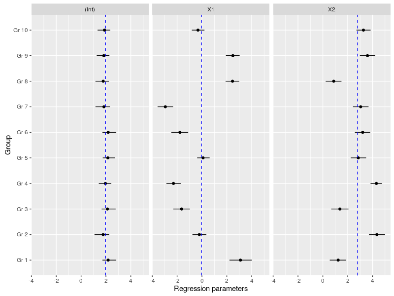
Another important plot is the variation in the regression parameters between the species, again this is easily done using the MCMC samples:

#now we could look at the variation in the regression coefficients between the groups doing caterpillar plots
ind_coeff<-apply(mcmc_hier$beta,c(2,3),quantile,probs=c(0.025,0.5,0.975))
df_ind_coeff<-data.frame(Coeff=rep(c("(Int)","X1","X2"),each=10),LI=c(ind_coeff[1,,1],ind_coeff[1,,2],ind_coeff[1,,3]),Median=c(ind_coeff[2,,1],ind_coeff[2,,2],ind_coeff[2,,3]),HI=c(ind_coeff[3,,1],ind_coeff[3,,2],ind_coeff[3,,3]))
gr<-paste("Gr",1:10)
df_ind_coeff$Group<-factor(gr,levels=gr)
#we may also add the population-level median estimate
pop_lvl<-data.frame(Coeff=c("(Int)","X1","X2"),Median=apply(mcmc_hier$gamma,2,quantile,probs=0.5))
ggplot(df_ind_coeff,aes(x=Group,y=Median))+geom_point()+
  geom_linerange(aes(ymin=LI,ymax=HI))+coord_flip()+
  facet_grid(.~Coeff)+
  geom_hline(data=pop_lvl,aes(yintercept=Median),color="blue",linetype="dashed")+
  labs(y="Regression parameters")

The cool thing with using STAN is that we can extend or modify the model in many ways. This will be the topics of future posts which will include: crossed and nested design, multilevel modelling, non-normal distributions and much more, stay tuned!

Code for the first plot:

cols<-brewer.pal(10,"Set3")
par(mfrow=c(1,2),mar=c(4,4,0,1),oma=c(0,0,3,5))
plot(y~X[,2],pch=16,xlab="Temperature",ylab="Response variable",col=cols[id])
lines(seq(-2,2,by=0.2),pred_x1[1,],lty=2,col="red")
lines(seq(-2,2,by=0.2),pred_x1[2,],lty=1,lwd=3,col="blue")
lines(seq(-2,2,by=0.2),pred_x1[3,],lty=2,col="red")
plot(y~X[,3],pch=16,xlab="Nitrogen concentration",ylab="Response variable",col=cols[id])
lines(seq(-2,2,by=0.2),pred_x2[1,],lty=2,col="red")
lines(seq(-2,2,by=0.2),pred_x2[2,],lty=1,lwd=3,col="blue")
lines(seq(-2,2,by=0.2),pred_x2[3,],lty=2,col="red")
mtext(text = "Population-level response to the two\nexplanatory variables with 95% CrI",side = 3,line = 0,outer=TRUE)
legend(x=2.1,y=10,legend=paste("Gr",1:10),ncol = 1,col=cols,pch=16,bty="n",xpd=NA,title = "Group\nID")