Simulating SEMs: part 2 extensions

Back in May I published a first post which simulated simple Structural Equation Models (SEMs) to check the capacity of piecewieseSEM to deal with noise. At that time the verdict was pretty bleak: 90% of models were accepted even if they were just fitting noise. Since then I extended the code to include model fitted via another R package for SEMs: lavaan plus three different data generations. Before plunging into the results a few words on the main difference between lavaan and piecewieseSEM.

lavaan vs piecewieseSEM

The basic idea of lavaan is to take the modelled relations between the variables, derive the expected variance-covariance matrix between all variables and compare the expected against the observed variance-covariance matrix. If the two matrices are not too far away the model is accepted and inferences are drawn from the fitted relations between the variables. The criteria most often used to assess if the model fit is acceptable is the model fit statistic which test the difference between the expected and observed variance-covariance matrix. If the p-value of the test is larger than 0.05 the model is generally accepted.

piecewiseSEM takes a different approach. The idea is to evaluate all relations not included in the model, compute some conditional probabilities and the Fischer’s C statistics. If all important relations are included in the set of models then the p-value of Fischer’s C statistic should be high. So again piecewiseSEM models are generally accepted if the p-value of the test statistics is greater than 0.05.

I won’t dwell that much here on the advantages and disadvantages of both approaches. Briefly lavaan main disadvantage is that it assumes that the data are multivariate normal which is a pretty strong constraints, the main advantages of lavaan are that it allows modeling latent variables and can directly compute strength and significance of mediating/indirect effects. On the other hand the main disadvantages of piecewiseSEM is that it allow almost infinite freedom in the sets of models that can be combined making it harder to relate these so-called path models to concepts like causality and mechanisms (see this earlier post on that). The main advantage of piecewiseSEM is its flexibility one can model hierarchical structure or non-normal distributions.

The two approaches deserve being compared in their strength and weaknesses against simulated datasets.

About the simulations

You can find all the code at the end of this article. The basic idea is to create a matrix summarising the presence/absence of relations between a set of variables. From these SEM models are set. The data simulation can follow three different scenarios, (i) the data are completely random, there is no signal in it, (ii) the data simulation follows exactly the set of relations indicated by the model, the data represent the model albeit with some added random variations, (iii) some of the causal relation are reversed, the model miht say that A -> B but the data follow B -> A. In addition to this variation the sample size (number of data points) vary from 20 to 100 and the number of variables vary from 5 to 10.

The data simulation and model fitting is done many times for the different sample size and number of variables values. At the end what is recorded is: (i) the proportion of models that would be accepted (p-value > 0.05), (ii) the proportion of paths/slopes that were significant, (iii) the average value of the significant paths.

Results

The first result is to look at the proportion of accepted models.

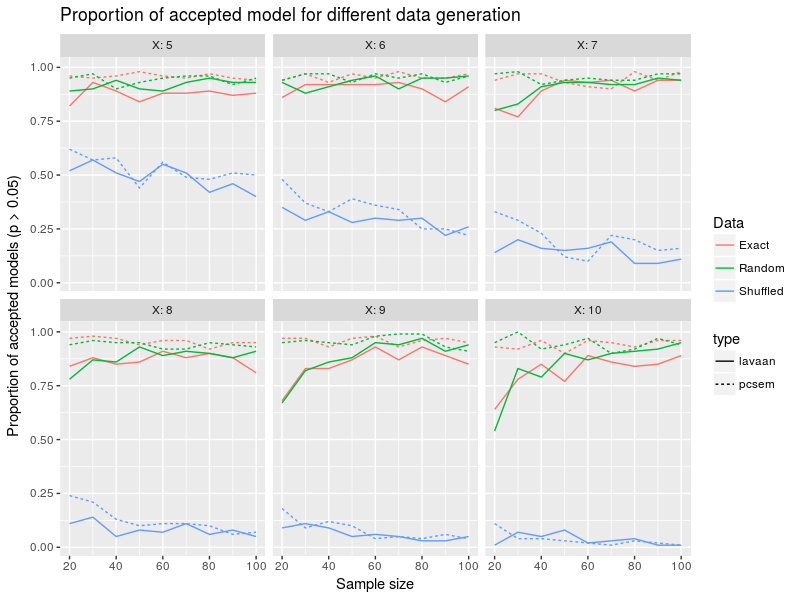
In this figure the colors represent the different data generation strategy (random, exact or shuffled), the linetype show the model fitting technique (lavaan or piecewieseSEM), the x-axis is the sample size, the different facets the number of variables in the model from 5 to 10 and the y-axis is the proportion of accepted models. The first intersting result is that the number of accepted models is pretty equivalent between the two approaches and is around 0.9 for both random and exact data generation. In other words whether you fitted just noise or some actual signal both lavaan and piecewiseSEM models will be accepted at a similar rate. More bluntly, the model test statistics used here are of no help to discriminate between models or to reject them. Interestingly as the number of variables included in the model increase, lavaan reject model more often for small sample sizes while piecewiseSEM acceptance rate is pretty constant overall cases. Shuffling causal relations leads to lower acceptance rate especially for high number of variables. Again piecewiseSEM and lavaan are pretty similar. In a nutshell, lavaan and piecewiseSEM have similar behvior regarding model acceptance, wrongly setting causal relation can lead to important drop in model acceptance but fitted to random data the models are accepted around 90% of the time.

Let’s turn to the second output, the proportion of significant paths:

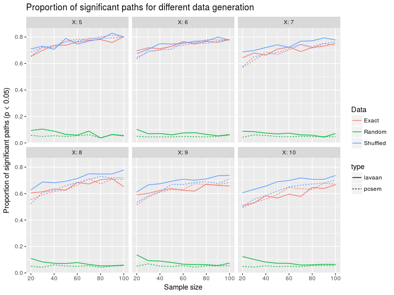
The structure of the figure is the same as before so can directly pluge into some interpretations. lavaan and piecewiseSEM patterns are again pretty close in this figure. There is a slight relation between sample size and proportion of singificant paths for exact and shuffled data generation, going from 20 to 100 data points increase proportion of significant paths from around 60 to 80%. With more variables in the model the average accepted proportion seem to decline, so more variables means less chance to detect (all) effects. The random data generation led to super-low proportions around 5-10% so close to the type I error rate. So it seems that accepting a model is no guarantee that there is something happening within the data, one needs to look at the relations (slopes) between the data. But there again getting significant slopes between variables does not tell whether the causal directions were correct, the model could say that A causes B when in fact B causes A in the data …

A final output is the average value of the significant paths:

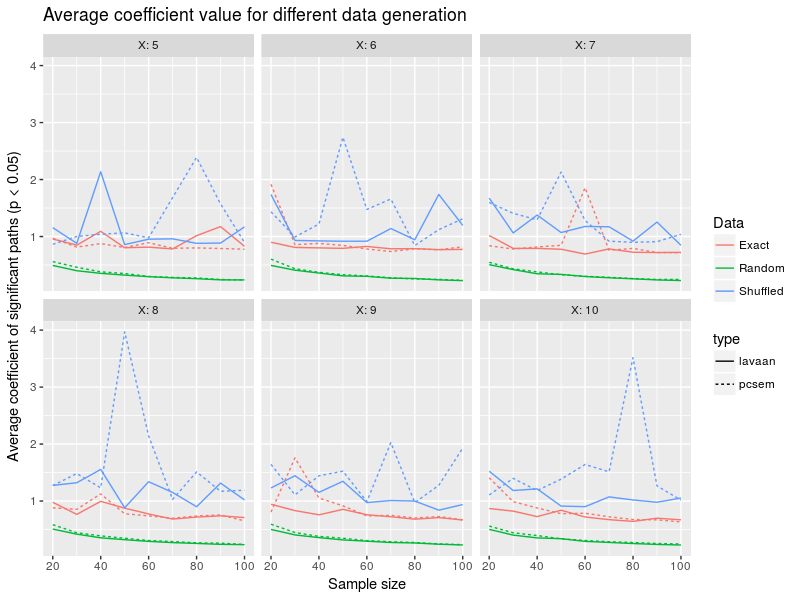
There is quite some noise in this figure, I might try later on the use the median rather than the mean, for some data simulations there were pretty large coefficient values mess up a bit with the lines. There is a slight decrease in the average path value for random data generation with sample size, meaning that as you collect more and more data, the significance threshold becomes easier to breach for smaller and smaller effects. Again lavaan and piecewiseSEM are pretty close together.

Conclusion

The main conclusion from this epxloration is that lavaan and piecewiseSEM are pretty identical, so use the one that fits closest to your need. Also the model test statistic is a poor indication that things are actually going on in your data so do not trust it. With relatively large sample size lavaan and piecewiseSEM have an adequate power of around 80% to detect effects between the variables yet there is no guarantee that you fitted the causal relations in the correct directions.

Next step for me would be to include some (hierarchical) structure in the data and simulate non-normal responses.

The code

Below is the full code, it is rather lengthy … Sorry for that.

library(piecewiseSEM)
library(lavaan)
library(dplyr)
library(ggplot2)

# create matrix with X variables with some relations indicated as ones
relation <- function(X=5,C=0.3){
  out <- matrix(0,nrow=X,ncol=X) #fill the matrix with 0s
  lwr <- X*(X-1)/2 #number of cells in the lower triangle of the matris
  nb.edge <- C*X**2 #number of 1s to add to the matrix
  if(nb.edge>lwr){
    stop("C is set too high to create a DAG, reduce it!")
  }
  while(!all(rowSums(out)[-1]!=0)){#while loop to ensure that all variables have at least one relation
    out <- matrix(0,nrow=X,ncol=X)
    out[lower.tri(out)][sample(x=1:lwr,size=nb.edge,replace=FALSE)] <- 1
    diag(out) <- 0 #ensure that no 1s are in the diagonal
  }
  rownames(out)<-paste0("X",1:X)
  return(out)
}

#turn a matrix with 0s and 1s into a series of R formulas
#rows are ys and columns are xs
formula_list <- function(mat){
  vars <- rownames(mat)
  formL <- list()
  for(i in 2:dim(mat)[1]){
    lhs <- vars[i] #the left-hand side of the formula
    rhs <- vars[mat[i,]==1] #the right-hand side of the formula
    if(length(rhs) == 0) { next }
    else{
      formL[[(i-1)]] <- formula(paste0(lhs,"~",paste(rhs,collapse="+")))
    }
  }
  return(formL[!sapply(formL,is.null)])
}

#turn a list of formulas into a list of models
model_list <- function(formL,data,fn=NULL){
  if(is.null(fn)){
    modL <- lapply(formL,function(x) lm(x,data))
  }
  else{
    stop("Not implemented yet") #one could allow the user to give a vector of model types
  }
  return(modL)
}

#create a function to get important infos from a sem object
grab_val <- function(modL,data,lavaan=FALSE){
  if(lavaan){
    lv <- "lavaan"
    semObj <- sem.lavaan(modL,data)
    sigM <-ifelse(!semObj@optim$converged,0,ifelse(semObj@test[[1]]$pvalue>=0.05,1,0)) #get the SEM p-value, giving a value of 0 if the model did not converged
    semCoeff <- parameterestimates(semObj)[grep("^~$",parameterestimates(semObj)$op),] #get the model coefficients
    nbPaths <- nrow(semCoeff)
    nbSigPaths <- length(which(semCoeff$pvalue<=0.05)) #how many significant paths
    avgSigPaths <- mean(abs(semCoeff$est[semCoeff$pvalue<=0.05])) #the average values of significant paths
  }
  else{
    lv <- "pcSEM"
    semObj <- sem.fit(modL,data,.progressBar = FALSE,conditional = TRUE) #evaluate the independence claims
    sigM <-ifelse(semObj$Fisher.C$p.value>=0.05,1,0) #get the SEM p-value
    semCoeff <- sem.coefs(modL,data) #get the model coefficients
    nbPaths <- nrow(semCoeff)
    nbSigPaths <- length(which(semCoeff$p.value<=0.05)) #how many significant paths
    avgSigPaths <- mean(abs(semCoeff$estimate[semCoeff$p.value<=0.05])) #the average values of significant paths
  }
  out <- data.frame(N=nrow(data),X=ncol(data),C=0.3,type=lv,sigM=sigM,nbPaths=nbPaths,nbSigPaths=nbSigPaths,avgSigPaths=avgSigPaths)
  return(out)
}
 
#a function to generate data based on diverse fidelity from the simulated list of models
generate_data <- function(N,X,relL,formL,type,p_shuffle){
  if(type=="random"){
    dat <- as.data.frame(matrix(rnorm(X*N,0,1),ncol=X,dimnames = list(1:N,paste0("X",1:X))))
  }
  else if(type=="exact"){
    dat <- data.frame(X1=runif(N,-2,2))
    for(f in formL){
      allv <- all.vars(f)
      y <- allv[1]
      xs <- dat[,allv[2:length(allv)]]
      xs <- as.matrix(cbind(rep(1,N),xs))
      coeff <- rcauchy(n = ncol(xs),0,2.5)
      dat<-cbind(dat,rnorm(N,xs%*%coeff,1))
      colnames(dat)[ncol(dat)]<-y
      dat <- as.data.frame(apply(dat,2,scale))
    }
  }
  #reverse a certain proportion of the causal relation, such as X1 -> X2 becomes X2 -> X1
  else if(type=="shuffled"){
    relL_m <- relL
    #how many relation to shuffle?
    #default to 0.25
    n_s <- ifelse(ceiling(sum(relL)*p_shuffle)<1,1,ceiling(sum(relL)*p_shuffle))
    #grab cell index to shuffle
    to_s <- sample(which(relL == 1),n_s,replace=FALSE)
    #grab row and column id for these cells
    id_s <- arrayInd(to_s,dim(relL))
    #transpose the 1s up the diagonal
    relL_m[id_s] <- 0
    relL_m[id_s[,c(2,1)]] <- 1
    #add column names
    dimnames(relL_m)[[2]] <- dimnames(relL_m)[[1]]
    if(!is_dag(graph_from_adjacency_matrix(relL_m))){
      while(!is_dag(graph_from_adjacency_matrix(relL_m))){
        #grab cell index to shuffle
        to_s <- sample(which(relL_m == 1),n_s,replace=FALSE)
        #grab row and column id for these cells
        id_s <- arrayInd(to_s,dim(relL))
        #transpose the 1s up the diagonal
        relL_m[id_s] <- 0
        relL_m[id_s[,c(2,1)]] <- 1
        #add column names
        dimnames(relL_m)[[2]] <- dimnames(relL_m)[[1]]
      }
    }
    #sort back the DAG
    od <- topo_sort(graph_from_adjacency_matrix(relL_m),mode="in")
    relL_mo <- relL_m[od,od]
    formL_m <- formula_list(relL_mo)
    #a random vector for the exogenous variable(s) to start of the data creation
    exo <- which(rowSums(relL_mo) == 0)
    dat <- as.data.frame(matrix(runif(N * length(exo),-2,2),ncol=length(exo)))
    names(dat) <- names(exo)
    for(f in 1:length(formL_m)){
      allv <- all.vars(formL_m[[f]])
      y <- allv[1]
      xs <- dat[,allv[2:length(allv)]]
      xs <- as.matrix(cbind(rep(1,N),xs))
      coeff <- rcauchy(n = ncol(xs),0,2.5)
      dat<-cbind(dat,rnorm(N,xs%*%coeff,1))
      colnames(dat)[ncol(dat)]<-y
      dat <- as.data.frame(apply(dat,2,scale))
    }
  }
  else{
    stop("Not implemented yet") #one could create datasets with non-random structure, to be implemented
  }
  return(dat)
}


#put it all in one function to replicate over
sim_sem <- function(N=20,X=5,C=0.3,type="random",p_shuffle = 0.25,lv=FALSE){
  relL <- relation(X=X,C=C)
  formL <- formula_list(relL)
  dat <- generate_data(N,X,relL,formL,type,p_shuffle)
  modL <- model_list(formL,dat)
  out <- grab_val(modL,dat,lavaan=lv)
  return(out)
}


#test over different sample size (N) and number of variables (X) with random data generation
#ie there is no simulated signal in the data
sims <- expand.grid(N=seq(20,100,10),X=5:10,C=0.3,lv=FALSE)
res <- NULL
for(i in 1:54){
  x <- as.numeric(sims[i,])
  tmp <- replicate(100,sim_sem(N = x[1],X=x[2],C=x[3],lv=x[4]))
  out <- as.data.frame(matrix(unlist(tmp),nrow = 100,byrow=TRUE,dimnames=list(1:100,attr(tmp,"dimnames")[[2]])))
  out$Exp <- i
  res <- rbind(res,out)
  print(i)
}
#now same stuff for lavaan
sims$lv<-TRUE
reslv <- NULL
for(i in 1:54){
  x <- as.numeric(sims[i,])
  tmp <- replicate(100,sim_sem(N = x[1],X=x[2],C=x[3],lv=x[4]))
  out <- as.data.frame(matrix(unlist(tmp),nrow = 100,byrow=TRUE,dimnames=list(1:100,attr(tmp,"dimnames")[[2]])))
  out$Exp <- i
  reslv <- rbind(reslv,out)
  print(i)
}
res$type<-"pcsem"
reslv$type<-"lv"
resa<-rbind(res,reslv)

resa%>%
  group_by(Exp,N,X,type)%>%
  summarise(PropSigM=sum(sigM,na.rm=TRUE)/n(),NbPaths = sum(nbPaths),NbSigPaths=sum(nbSigPaths),AvgSigPaths=mean(avgSigPaths,na.rm=TRUE))%>%
  mutate(PropSigPaths=NbSigPaths/NbPaths)->res_dd

#now simulate the exact distribution for the fitted model
sims <- expand.grid(N=seq(20,100,10),X=5:10,C=0.3,lv=FALSE)
res <- NULL
for(i in 1:54){
  x <- as.numeric(sims[i,])
  tmp <- replicate(100,sim_sem(N = x[1],X=x[2],C=x[3],lv=x[4],type="exact"))
  out <- as.data.frame(matrix(unlist(tmp),nrow = 100,byrow=TRUE,dimnames=list(1:100,attr(tmp,"dimnames")[[2]])))
  out$Exp <- i
  res <- rbind(res,out)
  print(i)
}
#now same stuff for lavaan
sims$lv<-TRUE
reslv <- NULL
for(i in 1:54){
  x <- as.numeric(sims[i,])
  tmp <- replicate(100,sim_sem(N = x[1],X=x[2],C=x[3],lv=x[4],type="exact"))
  out <- as.data.frame(matrix(unlist(tmp),nrow = 100,byrow=TRUE,dimnames=list(1:100,attr(tmp,"dimnames")[[2]])))
  out$Exp <- i
  reslv <- rbind(reslv,out)
  print(i)
}
res$type<-"pcsem"
reslv$type<-"lv"
resa<-rbind(res,reslv)
resa%>%
  group_by(Exp,N,X,type)%>%
  summarise(PropSigM=sum(sigM,na.rm=TRUE)/n(),NbPaths = sum(nbPaths),NbSigPaths=sum(nbSigPaths),AvgSigPaths=mean(avgSigPaths,na.rm=TRUE))%>%
  mutate(PropSigPaths=NbSigPaths/NbPaths)->res_dd2

#now simulate with shuffling the causal directions
sims <- expand.grid(N=seq(20,100,10),X=5:10,C=0.3,lv=FALSE)
res <- NULL
for(i in 1:54){
  x <- as.numeric(sims[i,])
  tmp <- replicate(100,sim_sem(N = x[1],X=x[2],C=x[3],lv=x[4],type="shuffled",p_shuffle = 0.25))
  out <- as.data.frame(matrix(unlist(tmp),nrow = 100,byrow=TRUE,dimnames=list(1:100,attr(tmp,"dimnames")[[2]])))
  out$Exp <- i
  res <- rbind(res,out)
  print(i)
}
#now same stuff for lavaan
sims$lv<-TRUE
reslv <- NULL
for(i in 1:54){
  x <- as.numeric(sims[i,])
  tmp <- replicate(100,sim_sem(N = x[1],X=x[2],C=x[3],lv=x[4],type="shuffled",p_shuffle = 0.25))
  out <- as.data.frame(matrix(unlist(tmp),nrow = 100,byrow=TRUE,dimnames=list(1:100,attr(tmp,"dimnames")[[2]])))
  out$Exp <- i
  reslv <- rbind(reslv,out)
  print(i)
}
res$type<-"pcsem"
reslv$type<-"lv"
resa<-rbind(res,reslv)
resa%>%
  group_by(Exp,N,X,type)%>%
  summarise(PropSigM=sum(sigM,na.rm=TRUE)/n(),NbPaths = sum(nbPaths),NbSigPaths=sum(nbSigPaths),AvgSigPaths=mean(avgSigPaths,na.rm=TRUE))%>%
  mutate(PropSigPaths=NbSigPaths/NbPaths)->res_dd3

#make one graph for all
res_all <- rbind(res_dd,res_dd2,res_dd3)
res_all$Data <- rep(c("Random","Exact","Shuffled"),each=108)
res_all$type[res_all$type=="lv"] <- "lavaan"

ggplot(res_all,aes(x=N,y=PropSigM,color=Data,linetype=type))+geom_path()+
  facet_wrap(~X,labeller = label_both) +
  labs(x="Sample size",y="Proportion of accepted models (p > 0.05)",
       title="Proportion of accepted model for different data generation")

ggplot(res_all,aes(x=N,y=PropSigPaths,color=Data,linetype=type))+geom_path()+
  facet_wrap(~X,labeller = label_both) +
  labs(x="Sample size",y="Proportion of significant paths (p < 0.05)",
       title="Proportion of significant paths for different data generation")

ggplot(res_all,aes(x=N,y=AvgSigPaths,color=Data,linetype=type))+geom_path()+
  facet_wrap(~X,labeller = label_both) +
  labs(x="Sample size",y="Average coefficient of significant paths (p < 0.05)",
       title="Average coefficient value for different data generation")