Correlation and Linear Regression in R

Before going into complex model building, looking at data relation is a sensible step to understand how your different variable interact together. Correlation look at trends shared between two variables, and regression look at causal relation between a predictor (independent variable) and a response (dependent) variable.

Correlation:

As mentionned above correlation look at global movement shared between two variables, for example when one variable increase (invalues) and the other increase as well, then these two variables are said to be positively correlated, the other way round when a variable increase and the other decrease then these two variables are negatively correlated. In the case of no correlation no pattern will be seen between the two variable.

Let’s look at some code before introducing correlation measure:

<span style="color:#0000ff;"><span style="font-family:Ubuntu Mono;"><span style="font-size:small;">> x<-sample(1:20,20)+rnorm(10,sd=2)</span></span></span>
<span style="color:#0000ff;"><span style="font-family:Ubuntu Mono;"><span style="font-size:small;">>y<-x+rnorm(10,sd=3)</span></span></span>
<span style="color:#0000ff;"><span style="font-family:Ubuntu Mono;"><span style="font-size:small;">> z<-(sample(1:20,20)/2)+rnorm(20,sd=5)</span></span></span>
<span style="color:#0000ff;"><span style="font-family:Ubuntu Mono;"><span style="font-size:small;">> df<-data.frame(x,y,z)</span></span></span>
<span style="color:#0000ff;"><span style="font-family:Ubuntu Mono;"><span style="font-size:small;">> plot(df[,1:3])</span></span></span>

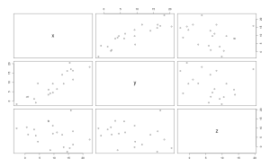
From the plot we get we see that when we plot the variable y with x, the points form some kind of line, when the value of x get bigger the value of y get somehow proportionnaly bigger too, we can suspect a positive correlation between x and y.

The measure of this correlation is called the coefficient of correlation and can calculated in different ways, the most usual measure is the Pearson coefficient, it is the covariance of the two variable divided by the product of their variance, it is scaled between 1 (for a perfect positive correlation) to -1 (for a perfect negative correlation), 0 would be complete randomness. We can get the Pearson coefficient of correlation using the function ‘cor’:

<span style="color:#0000ff;"><span style="font-family:Ubuntu Mono;"><span style="font-size:small;">> cor(df[,1:3],method="pearson")</span></span></span>
<span style="color:#000000;">        <span style="font-family:Ubuntu Mono;"><span style="font-size:small;">x          y          z</span></span></span>
<span style="color:#000000;"><span style="font-family:Ubuntu Mono;"><span style="font-size:small;">x  1.0000000  0.8736874 -0.2485967</span></span></span>
<span style="color:#000000;"><span style="font-family:Ubuntu Mono;"><span style="font-size:small;">y  0.8736874  1.0000000 -0.2376243</span></span></span>
<span style="color:#000000;"><span style="font-family:Ubuntu Mono;"><span style="font-size:small;">z -0.2485967 -0.2376243  1.0000000</span></span></span>
<span style="color:#0000ff;"><span style="font-family:Ubuntu Mono;"><span style="font-size:small;">> cor(df[,1:3],method="spearman")</span></span></span>
<span style="color:#000000;">        <span style="font-family:Ubuntu Mono;"><span style="font-size:small;">x          y          z</span></span></span>
<span style="color:#000000;"><span style="font-family:Ubuntu Mono;"><span style="font-size:small;">x  1.0000000  0.8887218 -0.3323308</span></span></span>
<span style="color:#000000;"><span style="font-family:Ubuntu Mono;"><span style="font-size:small;">y  0.8887218  1.0000000 -0.2992481</span></span></span>
<span style="color:#000000;"><span style="font-family:Ubuntu Mono;"><span style="font-size:small;">z -0.3323308 -0.2992481  1.0000000</span></span></span>

From these outputs our suspicion is confirmed x and y have a high positive correlation, but as always in statistics we can test if this coefficient is significant using parametric assumptions (Pearson, dividing the coefficient and its standard error, giving a value that follow a t-distribution) or when data violate parametric assumptions using Spearman rank coefficient.

<span style="color:#0000ff;"><span style="font-family:Ubuntu Mono;"><span style="font-size:small;">> cor.test(df$x,df$y,method="pearson")</span></span></span>

<span style="color:#000000;">        <span style="font-family:Ubuntu Mono;"><span style="font-size:small;">Pearson's product-moment correlation</span></span></span>

<span style="color:#000000;"><span style="font-family:Ubuntu Mono;"><span style="font-size:small;">data:  df$x and df$y </span></span></span>
<span style="color:#000000;"><span style="font-family:Ubuntu Mono;"><span style="font-size:small;">t = 7.6194, df = 18, p-value = 4.872e-07</span></span></span>
<span style="color:#000000;"><span style="font-family:Ubuntu Mono;"><span style="font-size:small;">alternative hypothesis: true correlation is not equal to 0 </span></span></span>
<span style="color:#000000;"><span style="font-family:Ubuntu Mono;"><span style="font-size:small;">95 percent confidence interval:</span></span></span>
<span style="color:#000000;"> <span style="font-family:Ubuntu Mono;"><span style="font-size:small;">0.7029411 0.9492172 </span></span></span>
<span style="color:#000000;"><span style="font-family:Ubuntu Mono;"><span style="font-size:small;">sample estimates:</span></span></span>
<span style="color:#000000;">      <span style="font-family:Ubuntu Mono;"><span style="font-size:small;">cor </span></span></span>
<span style="color:#000000;"><span style="font-family:Ubuntu Mono;"><span style="font-size:small;">0.8736874 </span></span></span>

<span style="color:#0000ff;"><span style="font-family:Ubuntu Mono;"><span style="font-size:small;">> cor.test(df$x,df$y,method="spearman")</span></span></span>

<span style="color:#000000;">        <span style="font-family:Ubuntu Mono;"><span style="font-size:small;">Spearman's rank correlation rho</span></span></span>

<span style="color:#000000;"><span style="font-family:Ubuntu Mono;"><span style="font-size:small;">data:  df$x and df$y </span></span></span>
<span style="color:#000000;"><span style="font-family:Ubuntu Mono;"><span style="font-size:small;">S = 148, p-value < 2.2e-16</span></span></span>
<span style="color:#000000;"><span style="font-family:Ubuntu Mono;"><span style="font-size:small;">alternative hypothesis: true rho is not equal to 0 </span></span></span>
<span style="color:#000000;"><span style="font-family:Ubuntu Mono;"><span style="font-size:small;">sample estimates:</span></span></span>
<span style="color:#000000;">      <span style="font-family:Ubuntu Mono;"><span style="font-size:small;">rho </span></span></span>
<span style="color:#000000;"><span style="font-family:Ubuntu Mono;"><span style="font-size:small;">0.8887218 </span></span></span>

An extension of the Pearson coefficient of correlation is when we square it we obtain the amount of variation in y explained by x (this is not true for the spearman rank based coefficient where squaring it has no statistical meanings). In our case we have around 75% of the variance in y that is explained by x.

However such results do not allow any causal explanation of the effect of x on y, indeed x could act on y in various way that are not always direct, all we can say from the correlation is that these two variables are linked somehow, to really explain and measure causal effect of x on y we need to use regression method, which will come next.

Linear Regression:

Regression is different from correlation because it try to put variables into equation and thus explain causal relationship between them, for exmple the most simple linear equation is written : Y=aX+b, so for every variation of unit in X, Y value change by a+b. Because we are trying to explain natural processes by equations that represent only part of the whole picture we are actually building a model that’s why linear regression are also called linear modelling.

In R we can build and test the significance of linear models.

<span style="color:#0000ff;"><span style="font-family:Ubuntu Mono;"><span style="font-size:small;">> m1<-lm(mpg~cyl,data=mtcars)</span></span></span>
<span style="color:#0000ff;"><span style="font-family:Ubuntu Mono;"><span style="font-size:small;">> summary(m1)</span></span></span>

<span style="color:#000000;"><span style="font-family:Ubuntu Mono;"><span style="font-size:small;">Call:</span></span></span>
<span style="color:#000000;"><span style="font-family:Ubuntu Mono;"><span style="font-size:small;">lm(formula = mpg ~ cyl, data = mtcars)</span></span></span>

<span style="color:#000000;"><span style="font-family:Ubuntu Mono;"><span style="font-size:small;">Residuals:</span></span></span>
<span style="color:#000000;">    <span style="font-family:Ubuntu Mono;"><span style="font-size:small;">Min      1Q  Median      3Q     Max </span></span></span>
<span style="color:#000000;"><span style="font-family:Ubuntu Mono;"><span style="font-size:small;">-4.9814 -2.1185  0.2217  1.0717  7.5186 </span></span></span>

<span style="color:#000000;"><span style="font-family:Ubuntu Mono;"><span style="font-size:small;">Coefficients:</span></span></span>
<span style="color:#000000;">            <span style="font-family:Ubuntu Mono;"><span style="font-size:small;">Estimate Std. Error t value Pr(>|t|)    </span></span></span>
<span style="color:#000000;"><span style="font-family:Ubuntu Mono;"><span style="font-size:small;">(Intercept)  37.8846     2.0738   18.27  < 2e-16 ***</span></span></span>
<span style="color:#000000;"><span style="font-family:Ubuntu Mono;"><span style="font-size:small;">cyl          -2.8758     0.3224   -8.92 6.11e-10 ***</span></span></span>
<span style="color:#000000;"><span style="font-family:Ubuntu Mono;"><span style="font-size:small;">---</span></span></span>
<span style="color:#000000;"><span style="font-family:Ubuntu Mono;"><span style="font-size:small;">Signif. codes:  0 ‘***’ 0.001 ‘**’ 0.01 ‘*’ 0.05 ‘.’ 0.1 ‘ ’ 1 </span></span></span>

<span style="color:#000000;"><span style="font-family:Ubuntu Mono;"><span style="font-size:small;">Residual standard error: 3.206 on 30 degrees of freedom</span></span></span>
<span style="color:#000000;"><span style="font-family:Ubuntu Mono;"><span style="font-size:small;">Multiple R-squared: 0.7262,     Adjusted R-squared: 0.7171 </span></span></span>
<span style="color:#000000;"><span style="font-family:Ubuntu Mono;"><span style="font-size:small;">F-statistic: 79.56 on 1 and 30 DF,  p-value: 6.113e-10</span></span></span>

The basic function to build linear model (linear regression) in R is to use the ‘lm’ function, you provide to it a formula in the form of y~x and optionally a data argument.

Using the ‘summary’ function we get all informations about our model: the formula called, the distribution of the residuals (the error of our models), the value of the coefficient and their significance plus an information on the overall model performance with the adjusted R-squared (0,71 in our case) that represent the amount of variation in y explained by x, so 71% of the variation in mpg can be explain by the variable cyl.

Before shouting ‘Eureka’ we should first check that the models assumptions are met, indeed linear models make a few assumptions on your data, the first one is that your data are normally distributed, the second one is that the variance in y is homogenous over all x values (sometimes called homoscedaticity) and independence which means that a y value at a certain x value should not influence other y values.

There is a marvellous built-in function to check all this:

<span style="color:#0000ff;"><span style="font-family:Ubuntu Mono;"><span style="font-size:small;">> par(mfrow=c(2,2))</span></span></span>
<span style="color:#0000ff;"><span style="font-family:Ubuntu Mono;"><span style="font-size:small;">> plot(m1)</span></span></span>

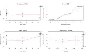
The ‘par’ argument is just to put all graphs in one window, the plot function is the real one.

The graphs on the first columns look at variance homogeneity among other things, normally you should see no pattern in the dots but just a random clouds of points. In this example this is clearly not the case since we see that the spreas of dots increase with higher values of cyl, our homogeneity assumptions is violated we can go back at the beginning and build new models this one cannot be interpreted… Sorry m1 you looked so great…

For the record the graph on the top right check the normality assumptions, if your data are normally distributed the point should fall (more or less) in a straight line, in this case the data are normal.

The final graph show how each y influence the model, each points is removed at a time and the new model is compared to the one with the point, if the point is very influential then it will have a high leverage value. Points with too high leverage value should be removed from the dataset to remove their outlying effect on the model.

Transforming the data;

There are a few basics mathematical transformations that can be applied to non normal or heterogenous data, usually it is a trial and error process;

<span style="color:#000000;"><span style="font-family:Ubuntu Mono;"><span style="font-size:small;"><span style="color:#0000ff;">> mtcars$Mmpg<-log(mtcars$mpg)</span></span></span></span>
<span style="color:#000000;"><span style="font-family:Ubuntu Mono;"><span style="font-size:small;"><span style="color:#0000ff;">> plot(Mmpg~cyl,mtcars)</span></span></span></span>

In our case this looks ok, but we can still remove the two outliers in ‘cyl’ categorie 8;

<span style="color:#0000ff;"><span style="font-family:Ubuntu Mono;"><span style="font-size:small;">n<-rownames(mtcars)[mtcars$Mmpg!=min(mtcars$Mmpg[mtcars$cyl==8])]</span></span></span>
<span style="color:#000000;"><span style="color:#0000ff;"><span style="font-family:Ubuntu Mono;"><span style="font-size:small;">mtcars2<-subset(mtcars,rownames(mtcars)%in%n)</span></span></span></span>

The first line ask for row names in ‘mtcars’ (rownames(mtcars)), but only return the one where the value of the variable ‘mpg’ is not equal (!=) to the minimum value of the variable ‘Mmpg’ which fall in the categorie of 8 cylinders. Then the list ‘n’ contain all these rownames and the next step is to make a new data frame that only contain rows with rownames present in the list ‘n’.

In this stage of transforming and removing outliers from the data you should use and abuse of plots to help you through the process.

Now let’s look back at our bivariate linear regression model from this new dataset;

<span style="color:#000000;"><span style="font-family:Ubuntu Mono;"><span style="font-size:small;"><span style="color:#0000ff;">> model<-lm(Mmpg~cyl,mtcars2)</span></span></span></span>
<span style="color:#000000;"><span style="font-family:Ubuntu Mono;"><span style="font-size:small;"><span style="color:#0000ff;">> summary(model)</span></span></span></span>

<span style="color:#000000;"><span style="font-family:Ubuntu Mono;"><span style="font-size:small;">Call:</span></span></span>
<span style="color:#000000;"><span style="font-family:Ubuntu Mono;"><span style="font-size:small;">lm(formula = Mmpg ~ cyl, data = mtcars2)</span></span></span>

<span style="color:#000000;"><span style="font-family:Ubuntu Mono;"><span style="font-size:small;">Residuals:</span></span></span>
<span style="color:#000000;">     <span style="font-family:Ubuntu Mono;"><span style="font-size:small;">Min       1Q   Median       3Q      Max </span></span></span>
<span style="color:#000000;"><span style="font-family:Ubuntu Mono;"><span style="font-size:small;">-0.19859 -0.08576 -0.01887  0.05354  0.26143 </span></span></span>

<span style="color:#000000;"><span style="font-family:Ubuntu Mono;"><span style="font-size:small;">Coefficients:</span></span></span>
<span style="color:#000000;">            <span style="font-family:Ubuntu Mono;"><span style="font-size:small;">Estimate Std. Error t value Pr(>|t|)    </span></span></span>
<span style="color:#000000;"><span style="font-family:Ubuntu Mono;"><span style="font-size:small;">(Intercept)  3.77183    0.08328  45.292  < 2e-16 ***</span></span></span>
<span style="color:#000000;"><span style="font-family:Ubuntu Mono;"><span style="font-size:small;">cyl         -0.12746    0.01319  -9.664 2.04e-10 ***</span></span></span>
<span style="color:#000000;"><span style="font-family:Ubuntu Mono;"><span style="font-size:small;">---</span></span></span>
<span style="color:#000000;"><span style="font-family:Ubuntu Mono;"><span style="font-size:small;">Signif. codes:  0 ‘***’ 0.001 ‘**’ 0.01 ‘*’ 0.05 ‘.’ 0.1 ‘ ’ 1 </span></span></span>

<span style="color:#000000;"><span style="font-family:Ubuntu Mono;"><span style="font-size:small;">Residual standard error: 0.1264 on 28 degrees of freedom</span></span></span>
<span style="color:#000000;"><span style="font-family:Ubuntu Mono;"><span style="font-size:small;">Multiple R-squared: 0.7693,     Adjusted R-squared: 0.7611 </span></span></span>
<span style="color:#000000;"><span style="font-family:Ubuntu Mono;"><span style="font-size:small;">F-statistic: 93.39 on 1 and 28 DF,  p-value: 2.036e-10 </span></span></span>

<span style="color:#000000;"><span style="font-family:Ubuntu Mono;"><span style="font-size:small;"><span style="color:#0000ff;">> plot(model)</span></span></span></span>

Again we have highly significant intercept and slope, the model explain 76% of the variance in log(mpg) and is overall significant. Now we biologist are trained to love and worship ANOVA table, in R there are several way to do it (as always an easy and straightforward way and another with more possibilities for tuning);

<span style="color:#000000;"><span style="font-family:Ubuntu Mono;"><span style="font-size:small;"><span style="color:#0000ff;">> anova(model)</span></span></span></span>
<span style="color:#000000;"><span style="font-family:Ubuntu Mono;"><span style="font-size:small;">Analysis of Variance Table</span></span></span>

<span style="color:#000000;"><span style="font-family:Ubuntu Mono;"><span style="font-size:small;">Response: Mmpg</span></span></span>
<span style="color:#000000;">          <span style="font-family:Ubuntu Mono;"><span style="font-size:small;">Df  Sum Sq Mean Sq F value    Pr(>F)    </span></span></span>
<span style="color:#000000;"><span style="font-family:Ubuntu Mono;"><span style="font-size:small;">cyl        1 1.49252 1.49252  93.393 2.036e-10 ***</span></span></span>
<span style="color:#000000;"><span style="font-family:Ubuntu Mono;"><span style="font-size:small;">Residuals 28 0.44747 0.01598   </span></span></span>
<span style="color:#000000;"><span style="font-family:Ubuntu Mono;"><span style="font-size:small;"><span style="color:#0000ff;">> library(car)</span></span></span></span>
<span style="color:#c5060b;"><span style="font-family:Ubuntu Mono;"><span style="font-size:small;">Le chargement a nécessité le package : MASS</span></span></span>
<span style="color:#c5060b;"><span style="font-family:Ubuntu Mono;"><span style="font-size:small;">Le chargement a nécessité le package : nnet</span></span></span>
<span style="color:#000000;"><span style="font-family:Ubuntu Mono;"><span style="font-size:small;"><span style="color:#0000ff;">> Anova(model)</span></span></span></span>
<span style="color:#000000;"><span style="font-family:Ubuntu Mono;"><span style="font-size:small;">Anova Table (Type II tests)</span></span></span>

<span style="color:#000000;"><span style="font-family:Ubuntu Mono;"><span style="font-size:small;">Response: Mmpg</span></span></span>
<span style="color:#000000;">           <span style="font-family:Ubuntu Mono;"><span style="font-size:small;">Sum Sq Df F value    Pr(>F)    </span></span></span>
<span style="color:#000000;"><span style="font-family:Ubuntu Mono;"><span style="font-size:small;">cyl       1.49252  1  93.393 2.036e-10 ***</span></span></span>
<span style="color:#000000;"><span style="font-family:Ubuntu Mono;"><span style="font-size:small;">Residuals 0.44747 28</span></span></span>

The second function (‘Anova’) allow you to define which type of sum-of-square you want to calculate (here is a nice explanation of their different assumptions) and also to correct for variance heterogeneity;

<span style="color:#000000;"><span style="font-family:Ubuntu Mono;"><span style="font-size:small;"><span style="color:#0000ff;">> Anova(model,white.adjust=TRUE)</span></span></span></span>
<span style="color:#000000;"><span style="font-family:Ubuntu Mono;"><span style="font-size:small;">Analysis of Deviance Table (Type II tests)</span></span></span>

<span style="color:#000000;"><span style="font-family:Ubuntu Mono;"><span style="font-size:small;">Response: Mmpg</span></span></span>
<span style="color:#000000;">          <span style="font-family:Ubuntu Mono;"><span style="font-size:small;">Df      F    Pr(>F)    </span></span></span>
<span style="color:#000000;"><span style="font-family:Ubuntu Mono;"><span style="font-size:small;">cyl        1 69.328 4.649e-09 ***</span></span></span>
<span style="color:#000000;"><span style="font-family:Ubuntu Mono;"><span style="font-size:small;">Residuals 28</span></span></span>

You would have noticed that the p-value is a bit higher. This function is very usefull for unbalanced dataset (which is our case) but need to take care when formulating the model especially when there is more than one predictor variables since the type II sum of square assume that there is no interaction between the predictors.

To sum up, correlation is a nice first step to data exploration before going into more serious analysis and to select variable that might be of interest (anyway it always produce sexy and easy to interprete graphs which will make your supervisor happy), then the next step is to model the variable relationship and the most basic models are bivariate linear regression that put the relation between the response variable and the predictor variable into equation and testing this using the summary and anova function. Since linear regression make several assumptions on the data before interpreting the results of the model you should use the function plot and look if the data are normally distributed, that the variance is homogenous (no pattern in the residuals~fitted values plot) and when necessary remove outliers.

Next step will be using multiple predictors and looking at generalized linear models.