Adding standard errors for interaction terms

This is something that bugged me for some time, how do we add up standard errors? This is relevant when you fit a model with interaction terms and you are interested not only in the deviation between different categories in your data (like male, female juvenils) but also whether the effect of some covariates on the response differ from 0.

Let’s look at a simple example, say you recorded the number of trees in 4 areas of your city: in the north, east, south and west. And you want to see if the average income in the different area of the town influence the number of trees. You are not only interested in knowing whether income effect of tree number differ between the areas but also if the income effect is significant within individual areas.

Let’s simulate some data reflecting this particular example:

#some simulated data
dat <- data.frame(income_std=runif(100,-2,2),
  area=gl(n = 4,k=25,labels = c("North","East","South","West")))
modmat <- model.matrix(~income_std*area,dat)
coeff <- c(1,2,-0.5,1.2,0.6,-1.3,-0.2,2)
dat$tree_nb <- rnorm(100,mean = modmat%*%coeff,sd=1)
  
#fit the model 
(m <- lm(tree_nb~income_std*area,dat))
    
##    Call:
##    lm(formula = tree_nb ~ income_std * area, data = dat)
##    
##    Coefficients:
##     (Intercept) income_std areaEast areaSouth areaWest income_std:areaEast 
##     1.0441 2.2062 -0.3837 0.9858 0.7059 -1.9570 
##    income_std:areaSouth income_std:areaWest 
##     -0.5658 1.8735

To get the effect of income in the different areas, we just need to add the estimated coefficients, for example the slope of number of trees vs income in the west of the city is: 2.21 + 1.87 = 4.08. How do we get the standard error for this sum? Wikipedia is here to help, the variance of a sum is basically the sum of the variance plus two times the covariance, in an equation:

\[\sigma_{X+Y}^{2} = \sigma_{X}^{2} + \sigma_{Y}^{2} + 2 * Cov(X,Y)\]

If we want the standard error we just need to plug in the standard errors instead of the variance (the $latex \sigma$’s) and take the square root.

Now the standard error are readily available in the summary of a fitted model, and for the covariance you can access them using the vcov function. I made a little function that does it for you (code at the end of the post), you basically provide the name of the factor variable (name_f argument) and the name of the covariate (name_x argument). If you leave name_x empty the function will return the intercept for each levels. Here is how you would apply it in the example:

#compute the summed SE
(sum_se <- rbind(add_se(m,name_f = "area"),
                add_se(m,name_f = "area",name_x = "income_std")))
    
                          Coef        SE
areaEast             0.6603816 0.1997875
areaSouth            2.0298995 0.2008723
areaWest             1.7499887 0.2051546
income_std:areaEast  0.2491587 0.2051456
income_std:areaSouth 1.6403689 0.1740335
income_std:areaWest  4.0796633 0.1817601
  
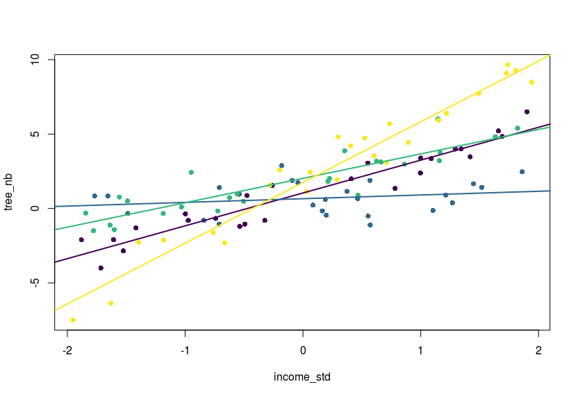
#a plot
library(viridis)
col_vec <- viridis(4)
plot(tree_nb~income_std,dat,pch=16,col=col_vec[dat$area])
abline(a = coef(m)[1],b=coef(m)[2],col=col_vec[1],lwd=2)
abline(a = sum_se[1,1],b=sum_se[4,1],col=col_vec[2],lwd=2)
abline(a = sum_se[2,1],b=sum_se[5,1],col=col_vec[3],lwd=2)
abline(a = sum_se[3,1],b=sum_se[6,1],col=col_vec[4],lwd=2)

Of course one could extend this to three-way or X-way interactions, you would just need to grab the relevant covariance values within the variance-covariance matrix returned by vcov.

Happy summing.

The code of the function, also available on github:

#function parameter
#@model: a lm or glm fitted model
#@name_f: a character string with the name of the categorical (factor) variable
#@name_x: a character string with the name fo the interacting variable, by default the intercept
add_se <- function(model,name_f,name_x="Intercept"){
  #grab the standard error of the coefficients
  se_vec <- summary(model)$coefficients[,2]
  if(name_x=="Intercept"){
    #the stabdard error of the intercept
    se_x <- se_vec[1]
    #get the level-specific standard errors
    se_f <- se_vec[grep(name_f,names(se_vec))]
    se_f <- se_f[-grep(":",names(se_f))]
    #get the covariance between the intercept and the level-specific parameters
    vcov_f <- vcov(model)[grep(name_f,rownames(vcov(model))),grep(name_x,colnames(vcov(model)))]
    vcov_f <- vcov_f[-grep(":",names(vcov_f))]
    #the estimated average value at each level
    coef_f <- coef(model)[1]+coef(model)[names(vcov_f)]
  }
  else{
    #similar code for the case of another variable than the intercept
    se_x <- se_vec[name_x]
    se_f <- se_vec[grep(name_f,names(se_vec))]
    se_f <- se_f[grep(":",names(se_f))]
    vcov_f <- vcov(model)[grep(name_f,rownames(vcov(model))),grep(name_x,colnames(vcov(model)))][,1]
    vcov_f <- vcov_f[grep(":",names(vcov_f))]
    coef_f <- coef(model)[name_x]+coef(model)[names(vcov_f)]
  }
  #compute the summed SE
  se_f <- sqrt(se_x**2+se_f**2+2*vcov_f)
  #create the output dataframe
  out <- data.frame(Coef=coef_f,SE=se_f)
  return(out)
}