Categorical random effects with lme4

The aim of this post is to see how to fit mixed effect models with varying effects when the explanatory variable that varies is a categorical variables. For instance imagine the following R formula:

\[y \sim X1 + (X1 | Group)\]

Where X1 is a categorical variable like sex, treatment or nationality.

First example: full factorial design

In this first example we will put together some simulated data from a full factorial design meaning that all groups (say all individuals) have data for all levels of the categorical variables. This can happen for example if you tested the speed of one operation from different workers using different kind of machines.

#load the libraries
library(MASS)
library(lme4)
library(lattice)
library(brms)
library(ggplot2)
library(gridExtra)
#a function to create appropriate variance-covariance matrices
#adapted from here: https://stats.stackexchange.com/questions/2746/how-to-efficiently-generate-random-positive-semidefinite-correlation-matrices
posDef <- function(d, k, corr = FALSE){
  W <- matrix(rnorm(d*k),ncol=k)
  S <- tcrossprod(W) 
  diag(S) <- diag(S) + runif(d)
  if(corr){
    S <- cov2cor(S)
  }
  return(S)
}

set.seed(20171105)
N <- 120 #number of observations
J <- 12 #number of workers

dat <- data.frame(Machine = factor(rep(letters[1:3],times=40))) 
modmat <- model.matrix(~.,dat) #the model matrix
dat$Ind_ID <- rep(1:J,each=N/J) #add the worker ID to the data frame
xtabs(~Ind_ID+Machine,dat) #to check the design
##       Machine
## Ind_ID a b c
##     1  4 3 3
##     2  3 4 3
##     3  3 3 4
##     4  4 3 3
##     5  3 4 3
##     6  3 3 4
##     7  4 3 3
##     8  3 4 3
##     9  3 3 4
##     10 4 3 3
##     11 3 4 3
##     12 3 3 4

#the coefficient for the regression
mu_b <- c(1,3,-4) #these are the population-level coefficients, the average operation time parameters
sigma_b <- posDef(3,2) #this is the variance-covariance matrix, how variable are the population-level coefficients
betas <- mvrnorm(n = J, mu = mu_b, Sigma = sigma_b) #sample for each worker the effect of working on the different machines
#the predicted values
linpred <- rowSums(modmat * betas[dat$Ind_ID,])
#simulate some response
dat$Time <- rnorm(N,linpred,1)

The tricky part to get at this point is the generation of the worker-level coefficients. One need to imagine that there is a population of worker out there and that there is some average operating time per machine types at the population-level. These average operating time is what we set in the mu_b object. Now, we assume that single worker would deviate from this population average and we encapsulate this deviation in the variance-covariance sigma_b matrix. A key point to note is that the operating time may not deviate independetly form one another. For example worker better than average with machine a might worse than average with machine b. This is what the covariance indicates.

A plot of the data might be helpful at this point:

ggplot(dat,aes(x=Ind_ID,y=Time,color=Machine))+geom_point()+
  stat_summary(fun.y=mean, geom="line") +
  coord_flip() +
  scale_x_continuous(breaks=1:12,labels=1:12) +
  geom_hline(yintercept = c(1,4,-3),color=c("red","green","blue"),linetype="dashed")

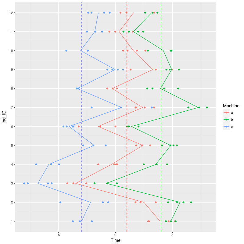
The dotted line show the population-level effect of the different machines, workers are, on average faster with machine b and slower on machine c. The solid line is joining the average values per machine across the different workers. We can see that, for instance, that Worker 3 is worse than average across all machines, Worker 1 show average operating time for machine b and c but much faster operating time on machine a.

In the model we want to have variation in the effect of machines on operating time for the different workers. There are two main ways to fit such a model, the first one is:

(m <- lmer(Time ~ Machine + (Machine | Ind_ID), dat))
## Linear mixed model fit by REML ['lmerMod']
## Formula: Time ~ Machine + (Machine | Ind_ID)
##    Data: dat
## REML criterion at convergence: 419.9672
## Random effects:
##  Groups   Name        Std.Dev. Corr       
##  Ind_ID   (Intercept) 2.0730              
##           Machineb    0.9329   -0.22      
##           Machinec    1.2394   -0.32  0.16
##  Residual             1.0605              
## Number of obs: 120, groups:  Ind_ID, 12
## Fixed Effects:
## (Intercept)     Machineb     Machinec  
##       1.029        2.687       -3.769

This model estimated for all parameters their variation between the workers (see the Std.Dev column above) plus the correlation in the varying effect. Basically this tells us that worker that were better than average on machine a tended to be a bit worst than average on machine b and c. We can compare the fitted correlation to the one we used to simulate our data:

cov2cor(sigma_b)
##            [,1]       [,2]        [,3]
## [1,]  1.0000000 0.17863836 -0.15839289
## [2,]  0.1786384 1.00000000  0.02149436
## [3,] -0.1583929 0.02149436  1.00000000

This might seem a bit far from the actual values that we fed in. One could look at the confidence intervals (using profile or bootMer) on these values to see how precise the estimates are.

Anyhow it is pretty costly and hard for a mixed effect model to estimate many variance-covariance parameters, one can quickly get into convergence warnings when the number of levels increase (remember that for N levels there is N * (N + 1) / 2 variance-covariance parameter to estimate). So an alternative model structure would be:

(m_2 <- lmer(Time ~ Machine + (1 | Ind_ID) + (1 | Ind_ID:Machine), dat))
## Linear mixed model fit by REML ['lmerMod']
## Formula: Time ~ Machine + (1 | Ind_ID) + (1 | Ind_ID:Machine)
##    Data: dat
## REML criterion at convergence: 421.1847
## Random effects:
##  Groups         Name        Std.Dev.
##  Ind_ID:Machine (Intercept) 0.8559  
##  Ind_ID         (Intercept) 1.8806  
##  Residual                   1.0616  
## Number of obs: 120, groups:  Ind_ID:Machine, 36; Ind_ID, 12
## Fixed Effects:
## (Intercept)     Machineb     Machinec  
##       1.032        2.682       -3.766

According to the github FAQ this random effect notation assume intercept varying among workers and among machines within workers (nested random effects). So the model will estimate for each worker a deviation from the average operating time, the model estimated that the standard deviation of these deviations was 1.88. In addition there will be an extra deviation for each worker on each machines, the model estimated that the standard deviation of these deviation was 0.86.

This model is simpler because it does not estimates the correlation between the varying effects, it assumes that workers are faster or slower on the machines in independant ways.

We can gather the model predictions and plot them against the data:

#get model prediction plus error taking into account individual variations
newdat <- data.frame(Machine=factor(letters[1:3]))
newdat$Time <- predict(m,newdat,re.form=NA) #this is the predicted average operating time per machines
mm <- model.matrix(~Machine,newdat)
var_eff <- diag(mm %*% tcrossprod(vcov(m),mm)) #the variation in the effect without taking into account worker effect
var_RE <- c(VarCorr(m)$Ind_ID[1,1],
            (VarCorr(m)$Ind_ID[1,1] + VarCorr(m)$Ind_ID[2,2] + 2 * VarCorr(m)$Ind_ID[2,1]),
            (VarCorr(m)$Ind_ID[1,1] + VarCorr(m)$Ind_ID[3,3] + 2 * VarCorr(m)$Ind_ID[3,1])) #the added worker effect
var_eff <- var_eff + var_RE
newdat$LCI <- newdat$Time - 2 * sqrt(var_eff) #the lower 95% CI bond
newdat$UCI <- newdat$Time + 2 * sqrt(var_eff) #the upper 95% CI bond
newdat$x <- c(1.1,2.1,3.1) #for easier plotting afterwards
newdat$Method <- "Full"
newdat <- rbind(newdat,newdat) #duplicate the dataframe for adding the results of the second model
newdat$Time[4:6] <- predict(m_2,newdat[4:6,],re.form=NA)
#for the second model the random effect structure is simpler we can just add the two random variation sources
var_eff <- diag(mm %*% tcrossprod(vcov(m_2),mm)) + c(VarCorr(m_2)$Ind_ID) + c(VarCorr(m_2)$`Ind_ID:Machine`)
newdat$LCI[4:6] <- newdat$Time[4:6] - 2 * sqrt(var_eff)
newdat$UCI[4:6] <- newdat$Time[4:6] + 2 * sqrt(var_eff)
newdat$x[4:6] <- c(0.9,1.9,2.9) #for easier plotting afterwards
newdat$Method[4:6] <- "Reduced"

ggplot(dat,aes(x=Machine,y=Time))+geom_jitter()+
  geom_point(data=newdat,aes(x=x,color=Method))+
  geom_linerange(data=newdat,aes(x=x,ymin=LCI,ymax=UCI,color=Method))

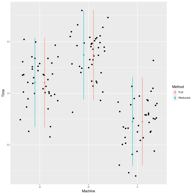
So for this particular dataset it did not appear worthwhile to actually estimate the extra covariance parameters. There is quite some discussion on which strategy one should adopt when chosing between alternative random effect structure, see the discussion and the article linked in the FAQ.

For this specific type of models if there is no inversion, like some the order of processing time per machines does not change across the workers (workers always work faster on machine b than on machine a and machine c). Then the simpler model, without covariation between the varying processing times between the machines, is a good choice.

On a side note, this particular data structure is well known in experimental biology / ecology, it is called split-plot design. You have a bunch of treatment that you want to apply to your plots and you basically sub-divide each plots into subplot and apply the treatments on the subplots. In the end each plot should get all treatments on its different subplots. There have been quite some efforts put into developping proper statistical methods (mainly in the ANOVA realm) for analyzing such data, but here we see that we can also analyze such data with lme4.

Second example: incomplete factorial design

Sometime we cannot have all levels of a categorical variable on each units. For instance a personn cannot be classified as both adult and teenager, or it might be unethical to expose test animals to all the drugs. In these cases we might still expect different units to respond differently to the categories and so want to fit similar models as before:

dat2 <- data.frame(Machine = factor(rep(letters[1:3],times=40))) 
modmat2 <- model.matrix(~.,dat2) #the model matrix
dat2$Ind_ID <- rep(1:J,times=N/J) #add the worker ID to the data frame
xtabs(~Ind_ID+Machine,dat2) #to check the design
##       Machine
## Ind_ID  a  b  c
##     1  10  0  0
##     2   0 10  0
##     3   0  0 10
##     4  10  0  0
##     5   0 10  0
##     6   0  0 10
##     7  10  0  0
##     8   0 10  0
##     9   0  0 10
##     10 10  0  0
##     11  0 10  0
##     12  0  0 10

#we will use the same coefficients as before
#the predicted values
linpred <- rowSums(modmat2 * betas[dat2$Ind_ID,])
#simulate some response
dat2$Time <- rnorm(N,linpred,1)

ggplot(dat2,aes(x=Ind_ID,y=Time,color=Machine))+geom_point()+
  stat_summary(fun.y=mean, geom="line") +
  coord_flip() +
  scale_x_continuous(breaks=1:12,labels=1:12) +
  geom_hline(yintercept = c(1,4,-3),color=c("red","green","blue"),linetype="dashed")

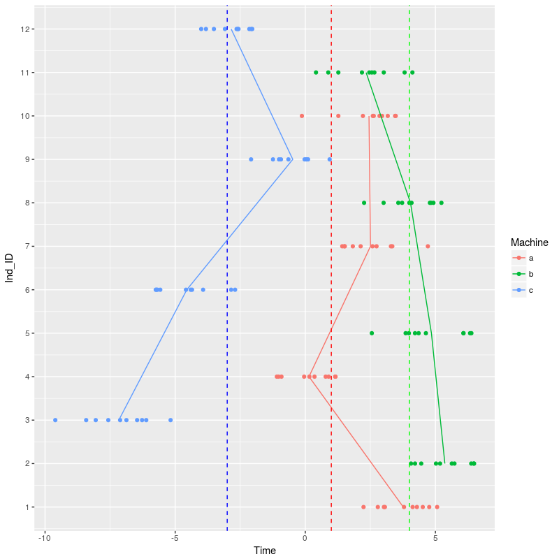
We can start to fit the same two models as before:

m_3 <- lmer(Time ~ Machine + (Machine | Ind_ID),dat2)
## Warning in checkConv(attr(opt, "derivs"), opt$par, ctrl = control
## $checkConv, : Hessian is numerically singular: parameters are not uniquely
## determined

The model did not fit due to some numerical issues, basically we do not have enough data to fit the complexity we are asking for with this model. One option is to go out and collect more data, another option is to try out a simpler model:

(m_4 <- lmer(Time ~ Machine + (1 | Ind_ID) + (1 | Ind_ID:Machine),dat2))
## Linear mixed model fit by REML ['lmerMod']
## Formula: Time ~ Machine + (1 | Ind_ID) + (1 | Ind_ID:Machine)
##    Data: dat2
## REML criterion at convergence: 386.2318
## Random effects:
##  Groups         Name        Std.Dev.
##  Ind_ID         (Intercept) 1.288   
##  Ind_ID:Machine (Intercept) 1.490   
##  Residual                   1.047   
## Number of obs: 120, groups:  Ind_ID, 12; Ind_ID:Machine, 12
## Fixed Effects:
## (Intercept)     Machineb     Machinec  
##       2.216        1.932       -5.978

This model worked. We can explore the random terms that were fitted with this model:

grid.arrange(dotplot(ranef(m_4,condVar=TRUE,whichel="Ind_ID"))[[1]],dotplot(ranef(m_4,condVar=TRUE,whichel="Ind_ID:Machine"))[[1]],ncol=2)

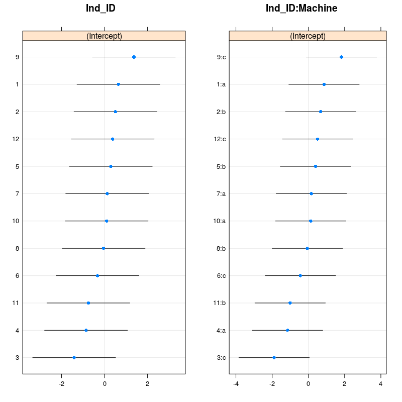
You can check with the figure above that indeed worker 9 was faster than average on machine c, while worker 3 was slower than average on machine c. Using the code from above one can also plot the model predictions:

newdat <- data.frame(Machine=factor(letters[1:3]))
newdat$Time <- predict(m_4,newdat,re.form=NA) #this is the predicted average operating time per machines
mm <- model.matrix(~Machine,newdat)
var_eff <- diag(mm %*% tcrossprod(vcov(m_4),mm)) + c(VarCorr(m_4)$Ind_ID) + c(VarCorr(m_4)$`Ind_ID:Machine`)
newdat$LCI <- newdat$Time - 2 * sqrt(var_eff) #the lower 95% CI bond
newdat$UCI <- newdat$Time + 2 * sqrt(var_eff) #the upper 95% CI bond

ggplot(dat,aes(x=Machine,y=Time))+geom_jitter()+
  geom_point(data=newdat,color="red")+
  geom_linerange(data=newdat,aes(ymin=LCI,ymax=UCI),color="red")

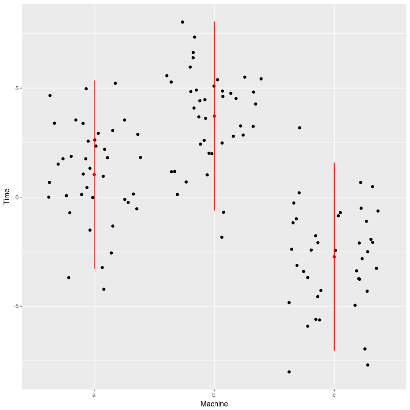
We see here that the model prediction are slightly off, especially for machine a, this is certainly due to small samples combined with large variations.

To wrap up: one can use categorical variables as varying terms in lme4 but one need to be aware of what the model specification means and if there are enough data to allow the model to fit. An important point here is that more data will not always solve the issue, for instance with the second example if we recorded worker 1 on machine a another 50 times this won’t help much further. More data help building more complex models when they fill some gaps, like when you ensure that all workers where recorded on all machines (at least one time).

This post is inspired by this presentation by Douglas Bates around slides 85-90.