Taking control of the legend in raster (in R)

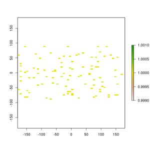
The basic default options of the raster package depict well continous data but when plotting caterogical data on maps like land use or species presence/absence other tricks should be used, below is some code to work around this.

<code class="r">library(raster)
## Loading required package: sp
## raster 2.0-41 (21-December-2012)


#create a raster of species presence/absence
r <- raster(nrows = 50, ncols = 50)
# randomly assign 100 cells as presence
id <- sample(1:2500, 100, replace = FALSE)
r[id] <- 1
# basic plotting
plot(r)
</code>

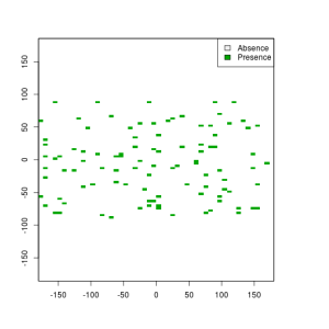
<code class="r"># customizing the legend
plot(r, legend = FALSE, col = rev(terrain.colors(2)))
legend("topright", legend = c("Absence", "Presence"), fill = rev(terrain.colors(2)))

`

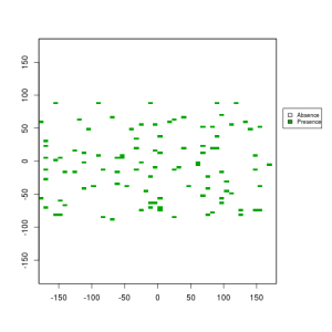
<code class="r"># to place the legend outside the map
par(xpd = FALSE)
plot(r, legend = FALSE, col = rev(terrain.colors(2)))
par(xpd = TRUE)
legend(x = 190, y = 80, legend = c("Absence", "Presence"), fill = rev(terrain.colors(2)), 
    cex = 0.7, inset = 0.9)
</code>

In these commands the legend argument on the plot function make the plot without legend, the col arguments set the colors here I use the reverse of the terrain colors palette (see ?plot::raster) Then in the legend function the first argument should be the position of the legend either as xy coords or as position like topright, bottom.. After that we need to set the names that will be present in the legend, the colors of the labels of the legend, the size of the character. Then the final arguments inset set the limit to which the element can be ploted on the graphic device. The par(xpd=) allow the ploting of object outside the scope of the graph.

Hope you enjoyed these.