Adding group-level predictors in GLMM using lme4

Sometime I happen to be wrong, this is one of these instance. The issue: a colleague measured individual plant growth and measured light irradiation received by each individual, the plants where in groups of 10 individuals and he measured soil parameters at the group-level. To analyze the effect of light on plant growth while controlling for soil and group variation, he built a mixed-effect model with group as a random term and light plus soil as fixed effect. As soil was measured at the group-level all individuals within a group got the same soil value.

When he came and asked if what he was doing was correct, I said that he had a classical multilevel dataset and that it was not possible to fit it using lme4, since the model would not know how to differentiate between variation explained by group effects and variation explained by soil effects. Actually this is possible, provided that the variable measured at the group-level is continuous (see this old post on a similar issue), one may add group-level predictors in lme4 fits. Let’s see how it works:

#load libraries
library(lme4)
library(ggplot2)
library(gridExtra)

#simulate some data

#first case one group-level predictor 
#and one individual level no interaction
  
#group-level predictor
soil <- runif(20,-2,2)
#individual level predictor
light <- runif(200,-2,2)
#group-level regression
grp_eff <- rnorm(20,2*soil,1)
#group index
group <- gl(n = 20,k = 10,
labels = letters[1:20])
#expected individual values
linpred <- 2 + grp_eff[group] + 2*light
#simulated individual values
growth <- rnorm(200,linpred,1)
#putting it together
dat <- data.frame(Group=group,Light=light,
Soil=soil[group],Growth=growth)
  
#model
(m <-lmer(Growth~Light+Soil+(1|Group),dat))

##Linear mixed model fit by REML ['lmerMod']
##Formula: Growth ~ Light + Soil + (1 | Group)
## Data: dat
##REML criterion at convergence: 608.1304
##Random effects:
## Groups Name Std.Dev.
## Group (Intercept) 0.6773 
## Residual 1.0046 
##Number of obs: 200, groups: Group, 20
##Fixed Effects:
##(Intercept) Light Soil 
## 2.354 2.042 2.122 

The parameter estimates looks pretty good, closed to the values used to simulate the data. It works! One can easily add group-level regression in lme4 provided that the group-level predictor(s) are continuous. Now we can make nice plots of the group and individual-level regressions.

#gather group-level deviation values 
#in one dataframe together with deviation
rf <- ranef(m,condVar=TRUE)
rff <- data.frame(Group=letters[1:20],Soil=soil,RF=rf$Group[,1],Var=attr(rf$Group,"postVar")[,,1:20])
#compute the group level regression
rff$RFF <- with(rff,RF+fixef(m)[2]*Soil)
#plot
p1 <- ggplot(rff,aes(x=Soil,y=RFF,ymin=RFF-2*Var,ymax=RFF+2*Var))+geom_point()+
 geom_abline(aes(intercept=0,slope=fixef(m)[2]))+geom_linerange()+
 labs(y="Group-level effect",title="Group-level regression")

#predict individual-level regression 
#for average group and average soil
newdat <- expand.grid(Light=seq(-2,2,length=20),Soil=0)
newdat$Pred <- predict(m,newdata=newdat,re.form=~0)
#plot
p2 <- ggplot(dat,aes(x=Light,y=Growth))+geom_point()+
 geom_line(data=newdat,aes(x=Light,y=Pred))+labs(title="Individual-level regression")
    
grid.arrange(p1,p2,ncol=2)

A word of caution now on using group-level regressions: I would be very careful (or better avoid) using p-values from such models. The degrees of freedom to test the soil effect are clearly inflated and are hard to guess, so I would advise against significance testing on the group-level regression. We can of course expand this approach to more complex situation (see some examples here), let’s see an example where we had an interaction between the group and the individual-level predictors:

#add interaction between group and individual-level 
#and unbalanced design

#group index
group <- factor(sample(letters[1:20],
         size = 200,replace=TRUE))
grp_eff <- rnorm(20,2*soil,1)

#expected individual values
linpred <- 2 + grp_eff[group] + 2 * light -  (grp_eff[group] * light)
#simulated individual values
growth <- rnorm(200,linpred,1)
#putting it together
dat <- data.frame(Group=group,Light=light,
       Soil=soil[group],Growth=growth)

#model
(m <-lmer(Growth~Light*Soil+(1|Group),dat))
    
    
##    Linear mixed model fit by REML ['lmerMod']
##    Formula: Growth ~ Light * Soil + (1 | Group)
##       Data: dat
##    REML criterion at convergence: 731.4661
##    Random effects:
##     Groups   Name        Std.Dev.
##     Group    (Intercept) 0.5474  
##     Residual             1.4182  
##    Number of obs: 200, groups:  Group, 20
##    Fixed Effects:
##    (Intercept)        Light         Soil   Light:Soil  
##          2.138        1.961        1.844       -1.865  

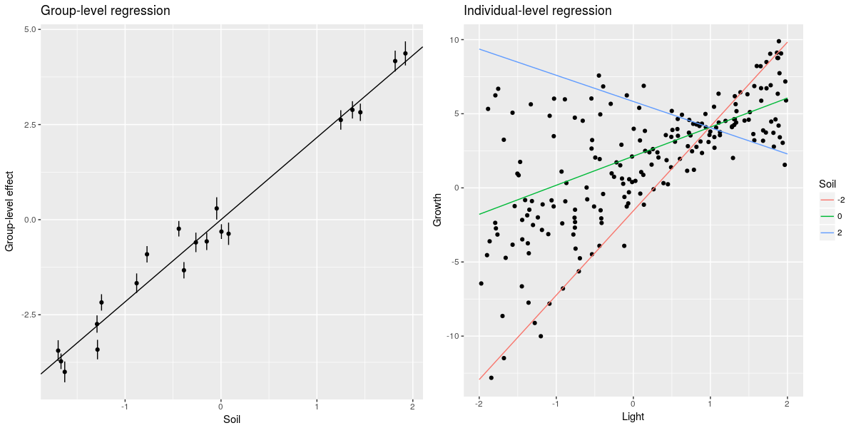
This is where it starts to get tricky for me, the estimate of the interaction between group and individual-level predictors is twice as big as the simulated value. Maybe I am doing something wrong in the simulation part … Anyhow we can still do some cool plots:

#group-level plot
rf <- ranef(m,condVar=TRUE)
rff <- data.frame(Group=letters[1:20],Soil=soil,RF=rf$Group[,1],Var=attr(rf$Group,"postVar")[,,1:20])
#compute the group level regression
rff$RFF <- with(rff,RF+2.16*Soil)
p1 <- ggplot(rff,aes(x=Soil,y=RFF,ymin=RFF-2*Var,ymax=RFF+2*Var))+geom_point()+
  geom_abline(aes(intercept=0,slope=2.16))+geom_linerange()+
  labs(y="Group-level effect",title="Group-level regression")

#predict individual effect for average group and average soil
newdat <- expand.grid(Light=seq(-2,2,length=20),Soil=c(-2,0,2))
newdat$Pred <- predict(m,newdata=newdat,re.form=~0)

p2 <- ggplot(dat,aes(x=Light,y=Growth))+geom_point()+
  geom_line(data=newdat,aes(x=Light,y=Pred,color=factor(Soil)))+
  labs(title="Individual-level regression")+
  scale_color_discrete(name="Soil")
  
grid.arrange(p1,p2,ncol=2)

That’s it, one does not need to use more complex modelling technique like maximum likelihood estimation or multilevel bayesian regression, one can use rather straightforward lme4 fits for exploring group-level regressions. A must-read for anyone interested in hierarchical/multilevel models is the Gelman and Hill book.