Exploring Spatial Patterns and Coexistance

Today is a rainy day and I had to drop my plans for going out hiking, instead I continued reading “Self-Organization in Complex Ecosystems” from Richard Solé and Jordi Bascompte.

As I will be busy in the coming weeks with spatial models at the iDiv summer school I was closely reading chapter three on spatial self-organization and decided to try and implement in R one of the Coupled Map Lattice Models that is described in the book.

The model is based on a discrete time version of the Lotka-Volterra competition model, for example for two competing species we model the population normalized abundances (the population abundance divided by the carrying capacity) N1 and N2 using the following equations:

$latex N_{1,t+1} = \phi_{N_{1}}(N_{1,t},N_{2,t}) = N_{1,t} * exp[r_{N_{1}} * (1 - N_{1} - \alpha_{12} * N_{2})] $

$latex N_{2,t+1} = \phi_{N_{2}}(N_{1,t},N_{2,t}) = N_{2,t} * exp[r_{N_{2}} * (1 - N_{2} - \alpha_{21} * N_{1})] $

Where r is the growth rate and the $latex \alpha$ are the interspecific competition coefficients. Note that since we use normalized abundance the intraspecific competition coefficient is equal to one.

Space can be introduced in this model by considering dispersion between neighboring cells. Say we have a 50 x 50 lattice map and that individuals disperse between neighboring cells with a probability D, as a result the normalized population abundances in cell k at time t+1 will be:

$latex N_{1,t+1,k} = (1 - D) * \phi_{N_{1}}(N_{1,t,k},N_{2,t,k}) + \frac{D}{8} * \sum_{j=1}^{8} \phi_{N_{1}}(N_{1,t,j},N_{2,t,j}) $

Where j is an index of all 8 neighboring cells around cell k. We have a similar equation for the competing species.

Now let’s implement this in R (you may a nicer version of the code here).

I start by defining two functions: one that will compute the population dynamics based on the first two equations, and the other one that will return for each cell in lattice the row numbers of the neighboring cells:

#Lotka-Voltera discrete time competition function
#@Ns are the population abundance
#@rs are the growth rate
#@as is the competition matrix
discrete<-function(Ns,rs,as){
  #return population abundance at time t+1
  return(as.numeric(Ns*exp(rs*(1-as%*%Ns))))
}

#an helper function returning line numbers of all neighbouring cells
find_neighbour<-function(vec,dat=dat){
  lnb<-which(dat[,"x"]%in%(vec["x"]+c(-1,-1,-1,0,1,1,1,0)) &
+ dat[,"y"]%in%(vec["y"]+c(-1,0,1,1,1,0,-1,-1)))
  #remove own line
  lnb<-lnb[which(lnb!=vec["lnb"])]
  return(lnb)
}

Then I create a lattice, fill it with the two species and some random noise.

dat<-expand.grid(x=1:50,y=1:50)
dat$N1<-0.5+rnorm(2500,0,0.1)
dat$N2<-0.5+rnorm(2500,0,0.1)
dat$lnb<-1:2500
list_dat<-list(dat)

The next step is to initialize all the parameters, in the example given in the book the two species have equal growth rate, equal dispersal and equal interspecific competition.

#competition parameters
as<-matrix(c(1,1.2,1.2,1),ncol=2,byrow=TRUE)
#growth rate
rs<-c(1.5,1.5)
#dispersal rate
ds<-c(0.05,0.05)
#infos on neighbouring cells
neigh<-apply(dat,1,function(x) find_neighbour(x,dat))

Now we are ready to start the model (the code is rather ugly, sorry for that, saturday coding makes me rather lazy …)

generation<-1:60
#model the dynamic assuming absorbing boundary (ie ind that go out of the grid are lost to the system)
for(i in generation){  
  list_dat[[(i+1)]]<-rbind.fill(apply(list_dat[[i]],1,function(x){
    #population dynamics within one grid cell
    intern<-(1-ds)*discrete(Ns=x[c("N1","N2")],rs=rs,as=as)
    #grab the neighbouring cells
    neigh_cell<-list_dat[[i]][neigh[[x["lnb"]]],]
    #the number of immigrant coming into the focal grid cell
    imm<-(ds/8)*rowSums(apply(neigh_cell,1,function(y) {
    discrete(Ns=y[c("N1","N2")],rs=c(1.5,1.5),as=as)}))
    out<-data.frame(x=x["x"],y=x["y"],N1=intern[1]+imm[1],N2=intern[2]
    + +imm[2],lnb=x["lnb"])
    return(out)
  }))
  #print(i)
}

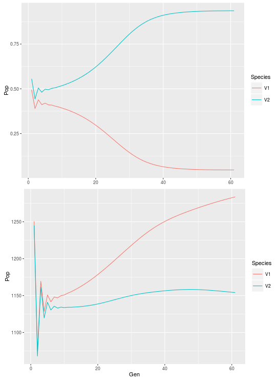
First let’s reproduce figure 3.8 from the book:

#look at coexistence between the two species within one cell
cell525<-ldply(list_dat,function(x) c(x[525,"N1"],x[525,"N2"]))
cell525$Gen<-1:61
cell525<-melt(cell525,id.vars="Gen",
+ measure.vars=1:2,variable.name="Species",value.name="Pop")
ggplot(cell525,aes(x=Gen,y=Pop,color=Species))+geom_path()

#look at coexistence across the system
all<-ldply(list_dat,function(x) c(sum(x[,"N1"]),sum(x[,"N2"])))
all$Gen<-1:61
all<-melt(all,id.vars="Gen",measure.vars=1:2,
+ variable.name="Species",value.name="Pop")
ggplot(all,aes(x=Gen,y=Pop,color=Species))+geom_path()

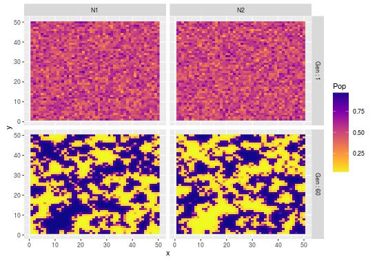
And now figure 3.9 plus an extra figure looking at the correlation in population abundance between the two species at the beginning and the end of the simulation:

#compare species-species abundance correlation at the beginning and at the end of the simulation
exmpl<-rbind(list_dat[[1]],list_dat[[60]])
exmpl$Gen<-rep(c("Gen : 1","Gen : 60"),each=2500)
ggplot(exmpl,aes(x=N1,y=N2))+geom_point()+facet_grid(.~Gen)

<img src="https://biologyforfun.files.wordpress.com/2016/06/space3.png" alt="space3" height="379" class="alignnone size-full wp-image-638" width="547"></img>

#look at variation in spatial patterns at the beginning and the end of the simulation
exmplm<-melt(exmpl,id.vars=c("x","y","Gen"),
+ measure.vars=c("N1","N2"),variable.name="Species",value.name="Pop")
ggplot(exmplm,aes(x,y,fill=Pop))+geom_raster()
 +scale_fill_viridis(option="plasma",direction=-1)+facet_grid(Gen~Species)

Neat stuff, I am looking forward to implement other models in this book!